2 Statistics
Product data science interviews tend to allocate 30 minutes to an hour for statistics problems. You will need to be proficient in the following:
- Hypothesis testing
- Central limit theorem
- Expectation estimation
- Variance, Covariance
- Everything we discussed in Chapter 1.
If you are preparing for PDS interviews you should study the excellent book on experiments by Kohavi, Tang, and Xu (2020).
2.1 Two-sample t-test
Question: What is a two-sample t-test?
Answer: A two-sample t-test tests whether there is a statistically significant difference between the means of two populations. Assume two samples, \(X_t, X_c\); for simplicity, let us call them control and treatment samples. We can define the difference of their means as: \(\Delta = \bar{X}_t - \bar{X_c}\). Then, the two-sample t-test can be written (p.186, Kohavi, Tang, and Xu (2020)) as:
\[ T = \frac{\Delta}{\sqrt{Var(\Delta)}} \]
Let’s expand on the previous relationship:
\[ T = \frac{ \bar{X}_t - \bar{X_c}}{\sqrt{Var(\bar{X}_t) + Var(\bar{X}_c) + 2COV(\bar{X}_t, \bar{X}_c)}} \] Since the two samples are independent, the covariance of the means is zero. The variance of the mean is:
\[ Var(X_t) = Var(\frac{X_1+X_2+X_{n_t}}{n_t}) = \frac{1}{n_t^2} \bigg[ Var(X_1) + Var(X_2) + ... \bigg] = \frac{n_t}{n_t^2} s_t^2 = \frac{s_t^2}{n_t} \]
where we assumed that all samples are independent and come from the same distribution, with empirical variance \(s_t^2\). Similarly, we can obtain the same result for the control group. Hence, our t-test can be written as:
\[ T = \frac{ \bar{X}_t - \bar{X_c}}{\sqrt{\frac{s_t^2}{n_t}+ \frac{s_c^2}{n_c}}} \]
2.2 Relationship between p-val and confidence interval
Question: What is the relationship between a p-value and a confidence interval?
Answer: A 95% confidence interval contains all values of a parameter, which if tested as null hypotheses, would give a P-value \(\geq 0.05\).
More often, we use the relationship between confidence intervals and p-values in an experimental setting, where we compare two quantities and the null hypothesis is that there is no difference. In this specific content, we can say that a 95% confidence interval of the treatment effect that does not overlap with zero implies a p-value of \(p < 0.05\).
2.3 Measuring sticks
Question: Assume there are two sticks with lengths \(l1\) and \(l2\). You have an instrument that can measure the length of a stick with an error \(e \in N(0,\sigma)\). Now assume that your budget constrains you to use the instrument only twice. What is the best way to use your budget in order to get the most accurate measurements?
Answer: The tricky part here is to realize that your goal is to minimize the variance of the measurement. The naive approach would be to measure \(l1\) and then \(l2\). In that case:
\[ \begin{align*} \hat{l1} &= l1 + e_1 \\ \hat{l2} &= l2 + e_2 \\ Var(\hat{l1}) &= Var(e_1)= \sigma^2 \\ Var(\hat{l2}) &= Var(e_2)= \sigma^2 \end{align*} \]
A better way to do this would be to measure the sum and the differences of the two:
\[ \begin{align*} \hat{m1} &= l1 + l2 + e_1 \\ \hat{m2} &= l2 - l1 + e_2 \\ \hat{l1} &= \frac{1}{2}(\hat{m1} - \hat{m2}) = l1 + \frac{1}{2}(e_1-e_2) \\ \hat{l2} &= \frac{1}{2}(\hat{m1} + \hat{m2}) = l2 + \frac{1}{2}(e_1+e_2) \\ Var(\hat{l1}) &= \frac{1}{4} [Var(e_1) + Var(e_2)] = \frac{1}{2}\sigma^2 \\ Var(\hat{l2}) &= \frac{1}{4} [Var(e_1) + Var(e_2)] = \frac{1}{2}\sigma^2 \end{align*} \]
In the above, the covariance of the two errors is zero since they are independent measurements.
2.4 Biased coin
Question: A coin was flipped 1000 times 550 of which turned out to be heads. Do you think this coin is biased?
Answer: We will solve this problem in two ways, both of which will invoke the Central Limit Theorem.
A. Solution through Binomial approximation: Assume that \(X_i\) represents a coin flip. The random variable \(\bar{X} = \sum_i X_i\) follows a Binomial distribution (sum of Bernoulli trials) and hence \(E[\bar{X}] = np\) and \(Var(\bar{X}) = np(1-p)\). Since the Binomial can be approximated by the Normal distribution, we can estimate the probability of observing 550 heads under the assumption (null hypothesis) that the coin is fair:
\[ \begin{align} Pr(X >= 550) &= 1 - Pr(X < 550) \\ &= 1 - Pr(Z < \frac{550-500}{\sqrt{250}}) \\ &= 1 - Pr(Z < 3.16) \approx 0.0008 \end{align} \] In the above, we standardized \(X\) to generate the Z statistic, even though it wasn’t necessary, and we used the Binomial’s mean and variance given above. Based on the above result, we can reject the Null hypothesis that the coin is fair since under the null, the probability of observing 550 heads or more would be almost zero.
If all of the above is confusing, you can always get an estimate directly from simulations:
## Standard normal: 0.0008## Original Binomial approximation: 0.0008A. Solution through Bernoulli trials and CLT: We can apply the Central Limit Theorem directly to the coin flips. Specifically, under the Null hypothesis that the coin is fair, we would expect that the mean probability of heads will follow a normal of \(N(0.5, \frac{0.5^2}{n}\). Then, similarly to what we did before:
\[ \begin{align} \Pr(X >= \frac{550}{1000}) &= 1- \Pr(X < 0.55) \\ &= 1 - \Pr(Z < \frac{0.55-0.5}{0.0158}) \\ &= 1 - \Pr(Z < 3.16) \approx 0.0008 \end{align} \]
2.5 Prussian horses
Question: The following dataset includes the number of deaths per year and corp:
## # A tibble: 6 × 3
##   deaths  year corp
##    <dbl> <dbl> <chr>
## 1      0    75 G
## 2      2    76 G
## 3      2    77 G
## 4      1    78 G
## 5      0    79 G
## 6 0 80 G## deaths year corp
## Min. :0.0 Min. :75.00 Length:280
## 1st Qu.:0.0 1st Qu.:79.75 Class :character
## Median :0.0 Median :84.50 Mode :character
## Mean :0.7 Mean :84.50
## 3rd Qu.:1.0 3rd Qu.:89.25
## Max. :4.0 Max. :94.00A. What kind of distribution does the number of deaths follow and with what parameters?
B. How would you test your response to question A?
C. If you had observed 4 deaths, could you reject the null that 4 deaths could be derived by the distribution of question A?
Answer:
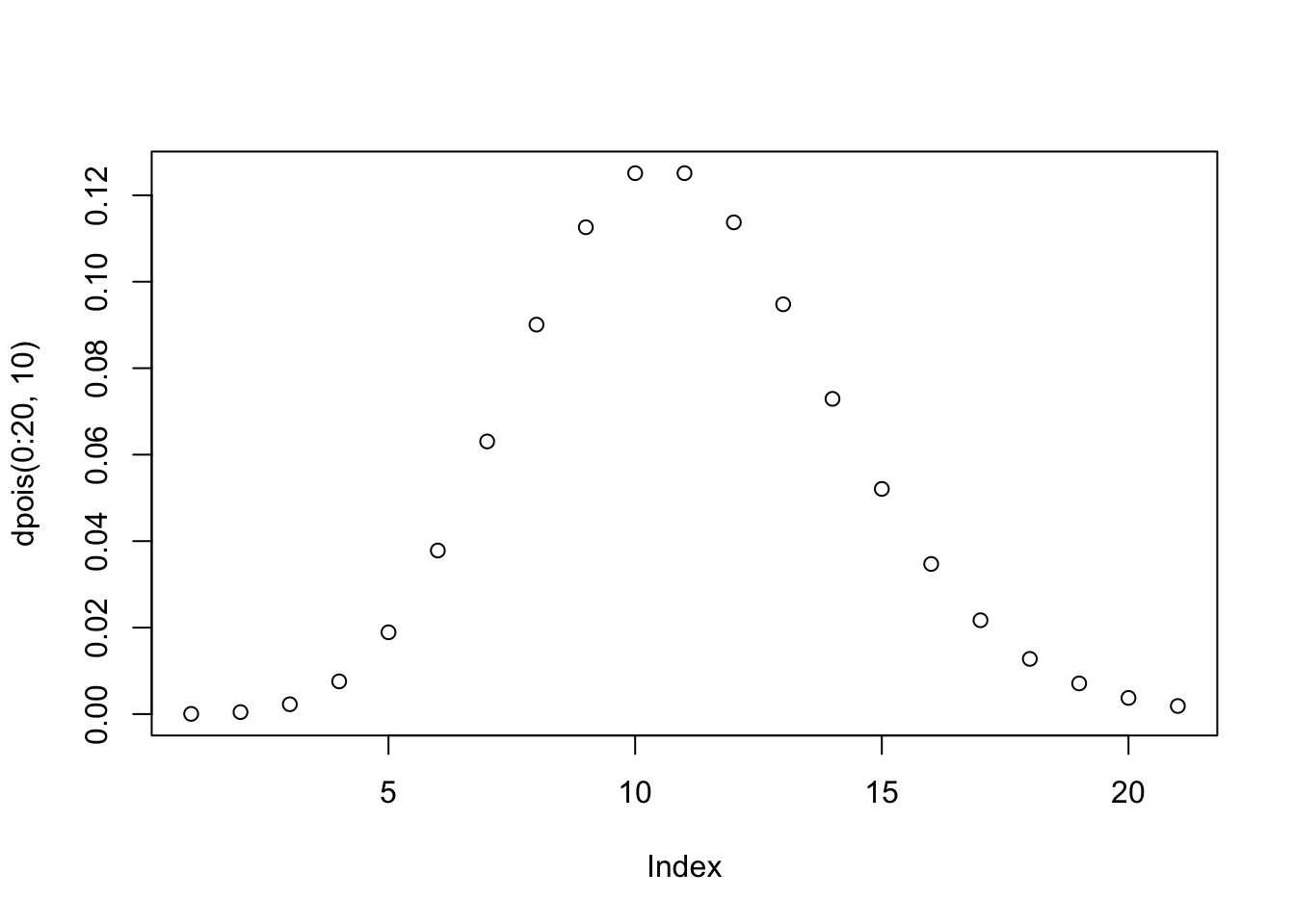
A. Given that we have positive integers, a natural choice would be to fit the number of deaths to a Poisson distribution, with \(\lambda = 0.7\) (see mean of data above). If we indeed do so, we can get the following:
lambda = 0.7
NumberOfObs = nrow(d)
predicted = c()
for(i in 0:4){
  prob = exp(-lambda) * lambda^i/factorial(i)
  cat(i,prob, " expected number of obs:", round(prob * NumberOfObs,1),
      " vs. actual obs: ", d %>% filter(deaths==i) %>% count %>% pull, "\n")
  predicted = c(predicted,round(prob * NumberOfObs) )
}
## 0 0.4965853 expected number of obs: 139 vs. actual obs: 144
## 1 0.3476097 expected number of obs: 97.3 vs. actual obs: 91
## 2 0.1216634 expected number of obs: 34.1 vs. actual obs: 32
## 3 0.02838813 expected number of obs: 7.9 vs. actual obs: 11
## 4 0.004967922 expected number of obs: 1.4 vs. actual obs: 2The predicted number of observations for each number of deaths is pretty close to the actually observed ones, so, just by looking at these numbers, we can feel confident that we made a good choice of distribution.
B. We can do a chi-squared test to see if there is statistical evidence that our data indeed follows a Poisson distribution:
##
##  Chi-squared test for given probabilities
##
## data:  actual
## X-squared = 2.7801, df = 4, p-value = 0.5953
The null hypothesis of the above test suggests that the two distributions are the same. We cannot reject the null, and hence it is statistically possible that this data was produced through a Poisson distribution.
C. The probability of observing 4 or more deaths assuming we the data follows a Poisson distribution with \(\lambda=0.7\) is equal to 0.00078, which is less than 0.05 (assuming significance level \(\alpha=0.05\)), and hence there is some evidence to reject the null hypothesis that the data can be model by this particular Poisson.
In R:
## 8e-04In Python:
## 0.0008
For instance:
What is the connection between Binomial and Poisson? The Poisson distribution is a limiting case of a Binomial distribution when the number of trials, n, gets very large and p, the probability of success, is small. As a rule of thumb, if \(n\geq 100\) and \(np \leq 10\), the Poisson distribution (taking \(\lambda=np\)) can provide a very good approximation to the binomial distribution.
You can find more here: https://math.oxford.emory.edu/site/math117/connectingPoissonAndBinomial/
When should you use Poisson vs. Binomial?
if the count (number of successes) has a ceiling/maximum value set by the experimental design, model the response as binomial (or some over/under-dispersed variant: quasibinomial, beta-binomial, observation-level random effect …)
if there is no well-defined limit (e.g., the number of trees in a 1-hectare plot can’t be infinite, but we can’t typically quantify the number of available “tree sites” that are available) then use a Poisson response (or some variant: quasi-Poisson, negative binomial, generalized Poisson, COM-Poisson …)
if the count has a maximum value but the proportion of the maximum is always small (e.g., the number of cancer cases in a county), then a binomial and a Poisson with a log-offset term to scale the maximum value will give nearly identical results, and it’s a matter of computational convenience.
When should you use Negative Binomial over Poisson?
- When we have a right-skewed distribution (the majority of points are clustered toward lower values of a variable) but also the variance is substantially higher than the mean!
2.6 Additional Questions
The following statistics questions are included in the complete book that defines the bar for product data science:
| Question | Topics |
|---|---|
| Confidence interval definition | Confidence interval, Hypothesis testing |
| P-value definition | P-value, Hypothesis testing |
| An intuitive way to write power | Power, Hypothesis testing |
| Tests for normality | Hypothesis testing, Normality |
| Confidence intervals that overlap | Confidence interval, Hypothesis testing |
| Manual estimation of flips | Normal, CDF, Binomial, CLT |
| CI of flipping heads | Confidence Interval, CLT, Bernoulli trials |
| Buy and sell stocks | Gambler ruin, Expectation, Recursion, Random walk |
| Expected number of consecutive heads | Expectation |
| Number of draws to get greater than 1 | Normal, Geometric, CDF, Expectation |
| Gambler’s ruin win probability | Gambler ruin, Random walk, Expectation |
| Distribution of a CDF | CDF, Inverse transform |
| Covariance of dependent variables | Variance, Uniform, Covariance, Expectation |
| Dynamic coin flips | Expectation, Simulation |
| Monotonic draws | Expectation |