第 2 章 基础模型
2.1 概述
统计模型计算的参数模型,并不是实际数据的关系,而是基于某原则(最小二乘,最大似然)最接近实际数据的模型。
2.2 热身
library(ggplot2)
library(dplyr)
##
## 载入程辑包:'dplyr'## The following objects are masked from 'package:stats':
##
## filter, lag## The following objects are masked from 'package:base':
##
## intersect, setdiff, setequal, unionlibrary(tidyr)
library(modelr)2.3 简单模型
用sim1的数据画图,观察数据分布。
ggplot(sim1, aes(x,y)) +
  geom_point()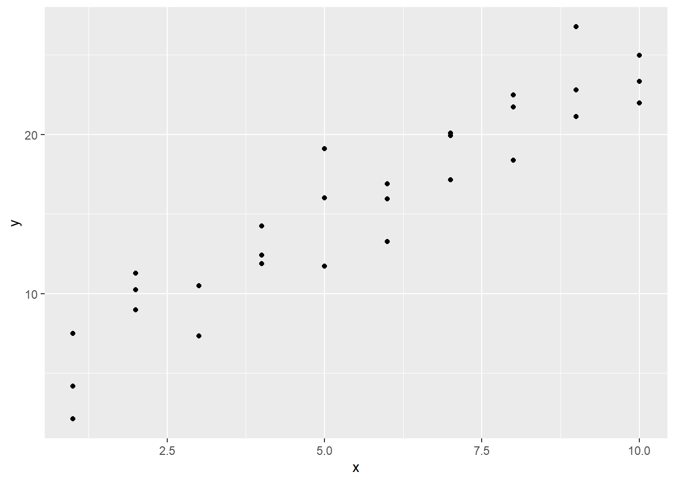
看起来随着变量X的增大,Y也增大,从形状来看二者具备线性关系,比如y = a0 + a1 * x。好了,开始建立一个模型,利用runif()函数随机生成a1, a2,将随机生成的a1,a2分配给`geom_abline()绘制线图看看。
models <- tibble(
  a1 = runif(250,-20,40),
  a2 = runif(250, -5,5)
)

ggplot(sim1, aes(x,y)) +
  geom_point() +
  geom_abline(data = models, aes(intercept = a1, slope = a2), alpha = 0.2)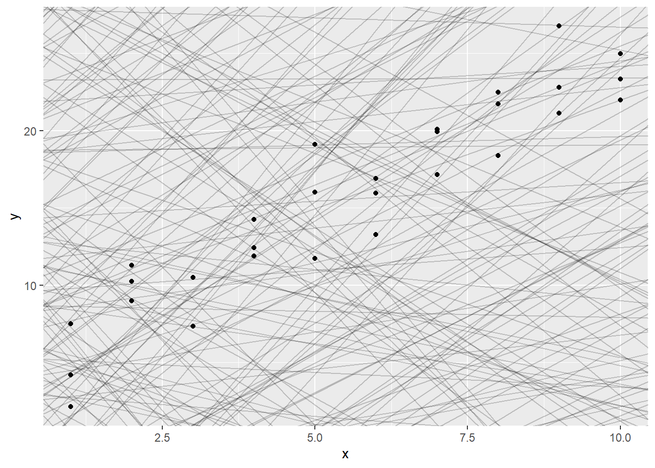
绘制了250条线,现在需要找到实际数据点距离模型距离最短的模型。
set.seed(1)
adj <- rnorm(30)
sim1 <- sim1 %>% mutate(x = x + adj)
distance <- tibble(x = sim1$x, y = sim1$y, xend = x, yend = 4.22 + 2.05 * x )
ggplot(sim1, aes(x,y)) +
  geom_point(alpha = 0.5) +
  geom_abline(aes(intercept = 4.22, slope = 2.05)) +
  geom_segment(data =distance, aes(x = x, y = y , xend = xend, yend = yend), col = "blue")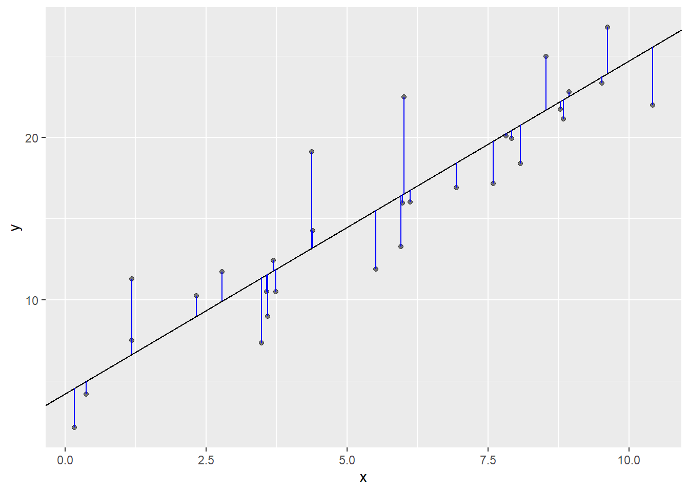
为了计算距离,创建1个函数,生成模型预测值。
model1 <- function(a, data){
  a[1] + a[2] * data$x
}

model1(c(3,6), sim1)
## [1] 5.241277 10.101860 3.986228 24.571685 16.977047 10.077190 23.924574
## [8] 25.429948 24.454688 25.167670 36.070687 29.339059 29.272557 19.711801
## [15] 39.749586 38.730398 38.902858 44.663017 49.927327 48.563408 50.513864
## [22] 55.692818 51.447390 39.063890 60.718954 56.663228 56.065227 54.175486
## [29] 60.131100 65.507649创建1个函数计算预测值与实际值之间的距离的残差
measure_dis <- function(mod, data){
  diff <- data$y - model1(mod,data)
  sqrt(mean(diff^2))
}

measure_dis(c(3,6), sim1)
## [1] 24.21746现在可以使用purrr计算250个模型的残差。
sim1_dist <- function(a1, a2){
  measure_dis(c(a1, a2),sim1)
}

models <- models %>%
  mutate(dist = purrr::map2_dbl(a1, a2, sim1_dist))
models %>% arrange(dist)
## # A tibble: 250 x 3
## a1 a2 dist
## <dbl> <dbl> <dbl>
## 1 1.97 2.44 2.96
## 2 7.94 1.41 3.06
## 3 7.87 1.62 3.10
## 4 2.38 2.02 3.17
## 5 1.50 2.59 3.21
## 6 8.59 1.58 3.41
## 7 1.28 2.83 3.94
## 8 9.76 1.57 4.15
## 9 -3.63 3.18 4.63
## 10 -0.608 2.18 4.75
## # ... with 240 more rows现在画出距离最短的10条线看看
ggplot(sim1, aes(x,y)) +
  geom_point(size = 2) +
  geom_abline(data = filter(models, rank(dist) <= 10)  , aes(intercept = a1, slope = a2, col = -dist))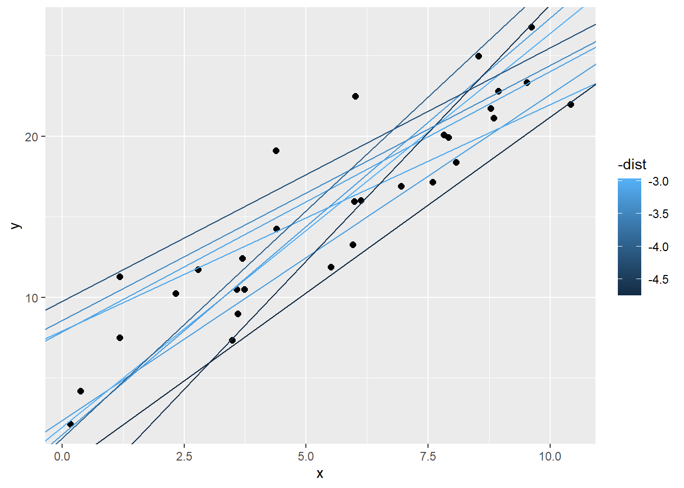
把模型的参数绘图
models %>% ggplot(aes(x = a1, y = a2, col = - dist)) +
  geom_point(data = filter(models, rank(dist) <= 10 ), aes(x = a1, y = a2), col = "red", size = 4) +
  geom_point() +
  stat_ellipse(type = "norm", level = 0.90)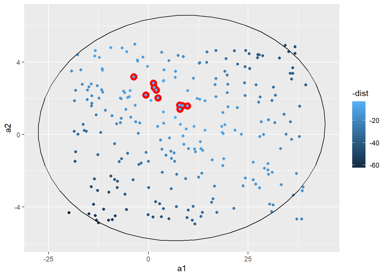
根据上图可以看出最合适的参数a1的分布范围在-5到20之间,a2在0到4之间,因此我们可以创建一个参数矩阵找到最合适的参数
grid <- expand.grid(
  a1 = seq(-5,20,length = 50),
  a2 = seq(0,4,length = 50)
) %>% mutate(
  dist = purrr::map2_dbl(a1, a2, sim1_dist)
)
grid %>% ggplot(aes(x = a1, y = a2)) +
  geom_point(data = filter(grid, rank(dist) <= 10), aes(x = a1, y = a2), size = 4, col = "red")+
  geom_point(aes(col = -dist))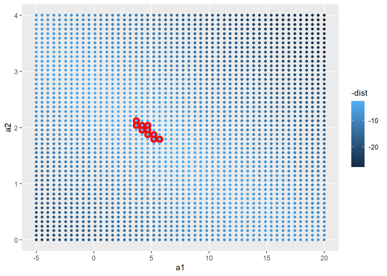
用最终获得的10个参数绘图
ggplot(sim1,aes(x = x, y = y )) +
geom_point() +
geom_abline(data = filter(grid, rank(dist) <= 10), aes(intercept = a1, slope = a2, col = - dist))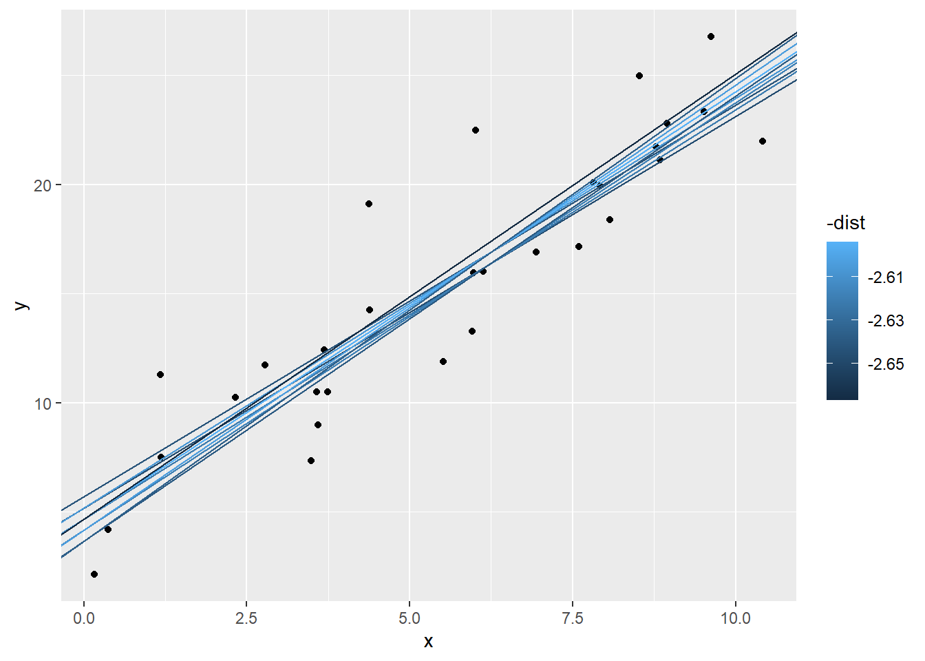 使用线性回归创建模型
sim1_mod <- lm(y ~ x, data = sim1)
coef(sim1_mod)
## (Intercept) x
## 4.587061 1.955625使用data_grid()生成样本空间
data(sim1)
grid <-  sim1 %>% data_grid(x)
生成预测值
grid <- grid %>% add_predictions(sim1_mod)
grid
## # A tibble: 10 x 2
## x pred
## <int> <dbl>
## 1 1 6.54
## 2 2 8.50
## 3 3 10.5
## 4 4 12.4
## 5 5 14.4
## 6 6 16.3
## 7 7 18.3
## 8 8 20.2
## 9 9 22.2
## 10 10 24.1使用真实值添加残差
sim1 <- sim1 %>% add_residuals(sim1_mod)
sim1
## # A tibble: 30 x 3
## x y resid
## <int> <dbl> <dbl>
## 1 1 4.20 -2.34
## 2 1 7.51 0.968
## 3 1 2.13 -4.42
## 4 2 8.99 0.491
## 5 2 10.2 1.74
## 6 2 11.3 2.80
## 7 3 7.36 -3.10
## 8 3 10.5 0.0514
## 9 3 10.5 0.0577
## 10 4 12.4 0.0250
## # ... with 20 more rows绘制残差密度分布图
sim1 %>% ggplot() +
  geom_freqpoly(aes(x = resid))
## `stat_bin()` using `bins = 30`. Pick better value with `binwidth`.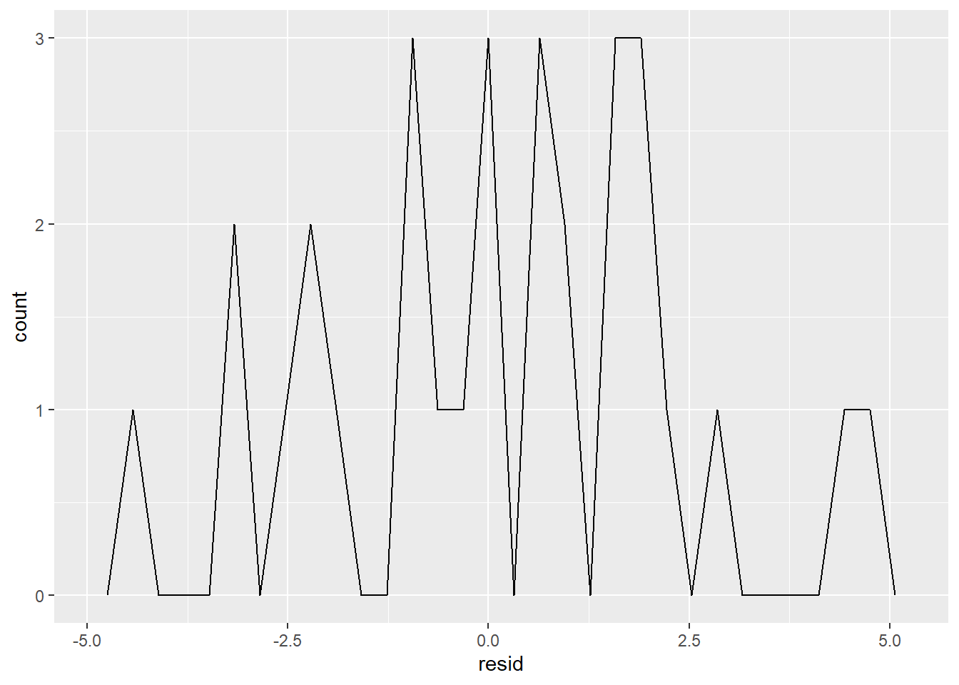
残差代替预测值的图
sim1 %>% ggplot(aes(x, resid)) +
  geom_ref_line(h = 0) +
  geom_point()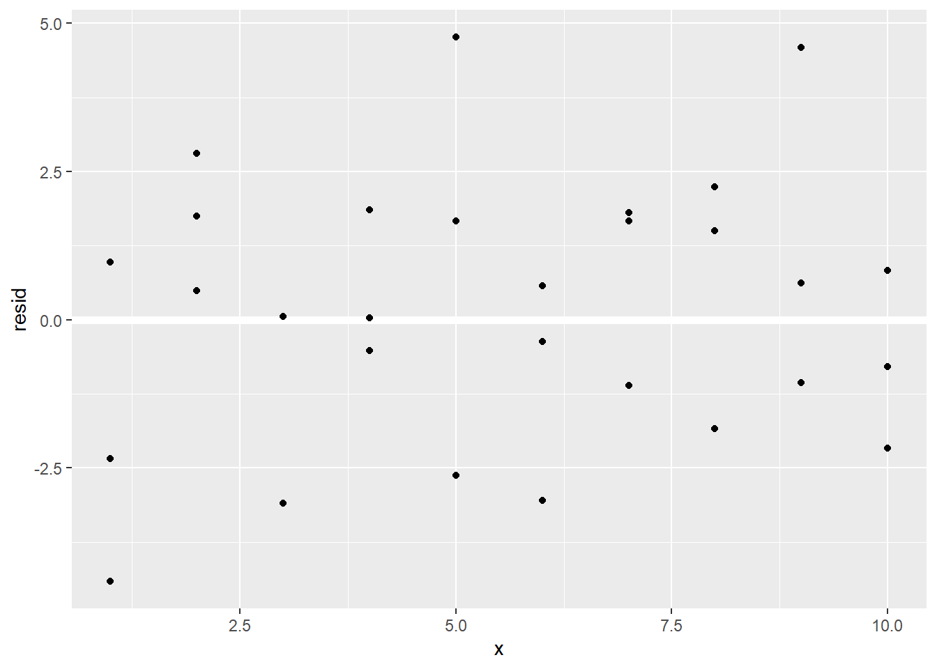
这些点看起来随机分布,提示模型预测效果较好。
2.3.1 练习
使用loess()曲线拟合sim1数据
data(sim1)
sim1_Mod2 <- loess(y ~ x, data = sim1)
sim1_Mod2 %>% summary()
## Call:
## loess(formula = y ~ x, data = sim1)
##
## Number of Observations: 30
## Equivalent Number of Parameters: 4.19
## Residual Standard Error: 2.262
## Trace of smoother matrix: 4.58 (exact)
##
## Control settings:
## span : 0.75
## degree : 2
## family : gaussian
## surface : interpolate cell = 0.2
## normalize: TRUE
## parametric: FALSE
## drop.square: FALSEgrid <- sim1 %>% data_grid(x) %>%
add_predictions(sim1_Mod2)
sim1 %>% ggplot(aes(x = x, y = y )) +
geom_point() +
geom_line(data = grid, aes(x = x ,y = pred),col = "blue", size = 3) +
geom_smooth(formula = y ~ x, col = "red", se = F, alpha = 0.2)## `geom_smooth()` using method = 'loess'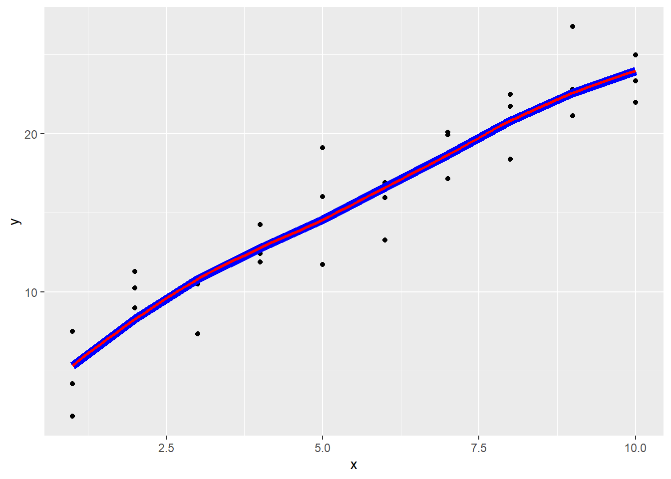
sim1 %>% spread_predictions(sim1_Mod2, sim1_mod)## # A tibble: 30 x 4
## x y sim1_Mod2 sim1_mod
## <int> <dbl> <dbl> <dbl>
## 1 1 4.20 5.34 6.54
## 2 1 7.51 5.34 6.54
## 3 1 2.13 5.34 6.54
## 4 2 8.99 8.27 8.50
## 5 2 10.2 8.27 8.50
## 6 2 11.3 8.27 8.50
## 7 3 7.36 10.8 10.5
## 8 3 10.5 10.8 10.5
## 9 3 10.5 10.8 10.5
## 10 4 12.4 12.8 12.4
## # ... with 20 more rows2.4 矩阵填充tribble
df <- tribble(
  ~y, ~x1, ~x2,
  4, 3, 5,
  5, 2, 6,
  6, 1, 7
)
df
## # A tibble: 3 x 3
## y x1 x2
## <dbl> <dbl> <dbl>
## 1 4 3 5
## 2 5 2 6
## 3 6 1 7model_matrix(df, y ~ x1 + x2 )## # A tibble: 3 x 3
## `(Intercept)` x1 x2
## <dbl> <dbl> <dbl>
## 1 1 3 5
## 2 1 2 6
## 3 1 1 72.5 分类变量模型
当使用分类变量作为因变量的时候,字符型变量无法参与计算。在R中将factor默认转换为数字计算。例如factor(c("男" ,"女"))将男和女分别转换为0,1进行计算。
df <- tribble(
  ~ sex, ~ response,
  "male", 1,
  "female", 2,
  "male", 1
)

model.matrix(data = df, response ~ sex)
## (Intercept) sexmale
## 1 1 1
## 2 1 0
## 3 1 1
## attr(,"assign")
## [1] 0 1
## attr(,"contrasts")
## attr(,"contrasts")$sex
## [1] "contr.treatment"使用sim2的数据建模,观察一下数据分布
data("sim2")
ggplot(sim2,aes(x, y)) + geom_point()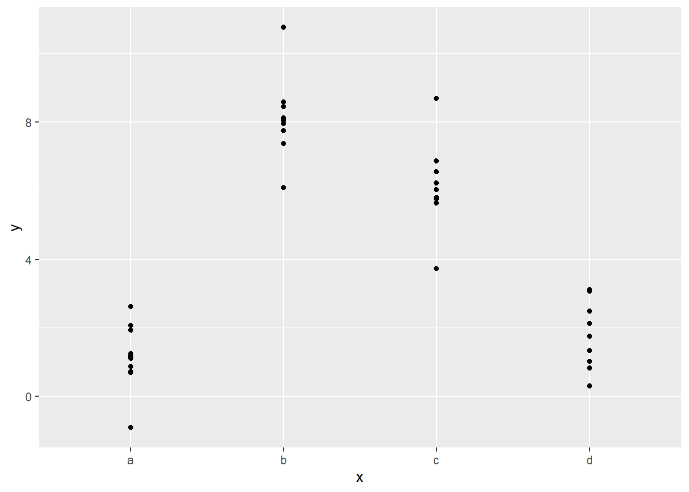
使用线性模型拟合
mod2 <-  lm(y ~ x, data = sim2)
grid <- sim2 %>%
  data_grid(x) %>%
  add_predictions(mod2)
grid
## # A tibble: 4 x 2
## x pred
## <chr> <dbl>
## 1 a 1.15
## 2 b 8.12
## 3 c 6.13
## 4 d 1.91看看模型预测值的分布
ggplot(sim2,aes(x, y)) +
  geom_point(data = grid, aes(x, pred), col = "red", size = 4) +
  geom_point()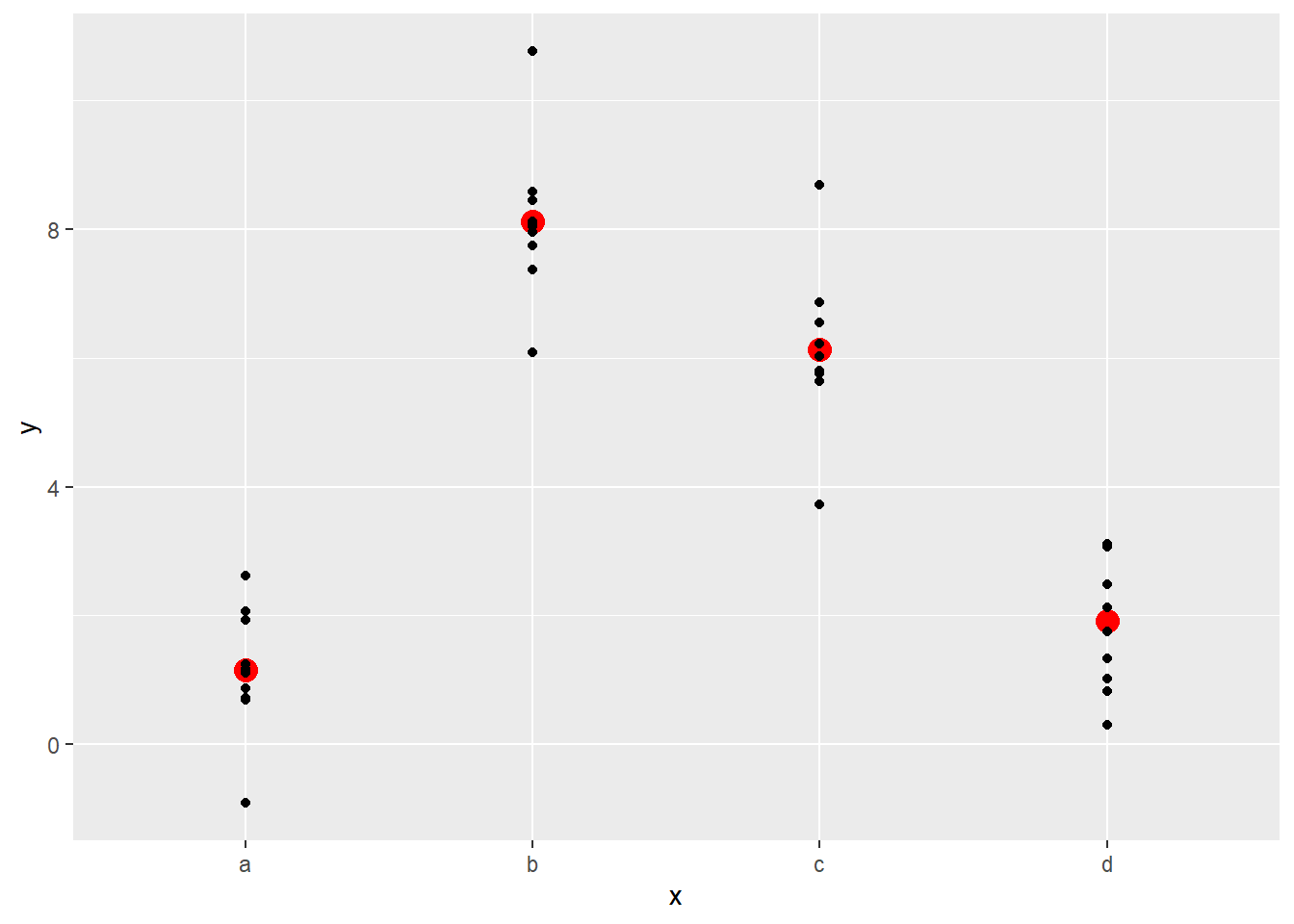
看起来预测的值是自变量的均值。注意: 无法使用未观测的自变量在模型中预测。