第 5 章 复杂模型
三个目标:
1. 使用简单模型来理解复杂模型。
2. 使用list-columns(列表列)在数据框中储存数据。
3. 使用broom包来整理模型结果。
5.1 gamminder数据分析
library(gapminder)
library(tidyverse)
## -- Attaching packages --------------------------------------- tidyverse 1.3.1 --## v ggplot2 3.3.5 v purrr 0.3.4
## v tibble 3.1.6 v dplyr 1.0.7
## v tidyr 1.1.4 v stringr 1.4.0
## v readr 2.1.1 v forcats 0.5.1## -- Conflicts ------------------------------------------ tidyverse_conflicts() --
## x dplyr::filter() masks stats::filter()
## x dplyr::lag() masks stats::lag()library(modelr)
gapminder## # A tibble: 1,704 x 6
## country continent year lifeExp pop gdpPercap
## <fct> <fct> <int> <dbl> <int> <dbl>
## 1 Afghanistan Asia 1952 28.8 8425333 779.
## 2 Afghanistan Asia 1957 30.3 9240934 821.
## 3 Afghanistan Asia 1962 32.0 10267083 853.
## 4 Afghanistan Asia 1967 34.0 11537966 836.
## 5 Afghanistan Asia 1972 36.1 13079460 740.
## 6 Afghanistan Asia 1977 38.4 14880372 786.
## 7 Afghanistan Asia 1982 39.9 12881816 978.
## 8 Afghanistan Asia 1987 40.8 13867957 852.
## 9 Afghanistan Asia 1992 41.7 16317921 649.
## 10 Afghanistan Asia 1997 41.8 22227415 635.
## # ... with 1,694 more rows这部分我们主要关注3个变量(lifeExp),(year)和(country),以回答一个问题:预期寿命与时间和国家有什么样的关系?先画个图观察一下这几个变量:
gapminder %>% ggplot(aes(x = year, y = lifeExp, group = country)) +
  geom_line()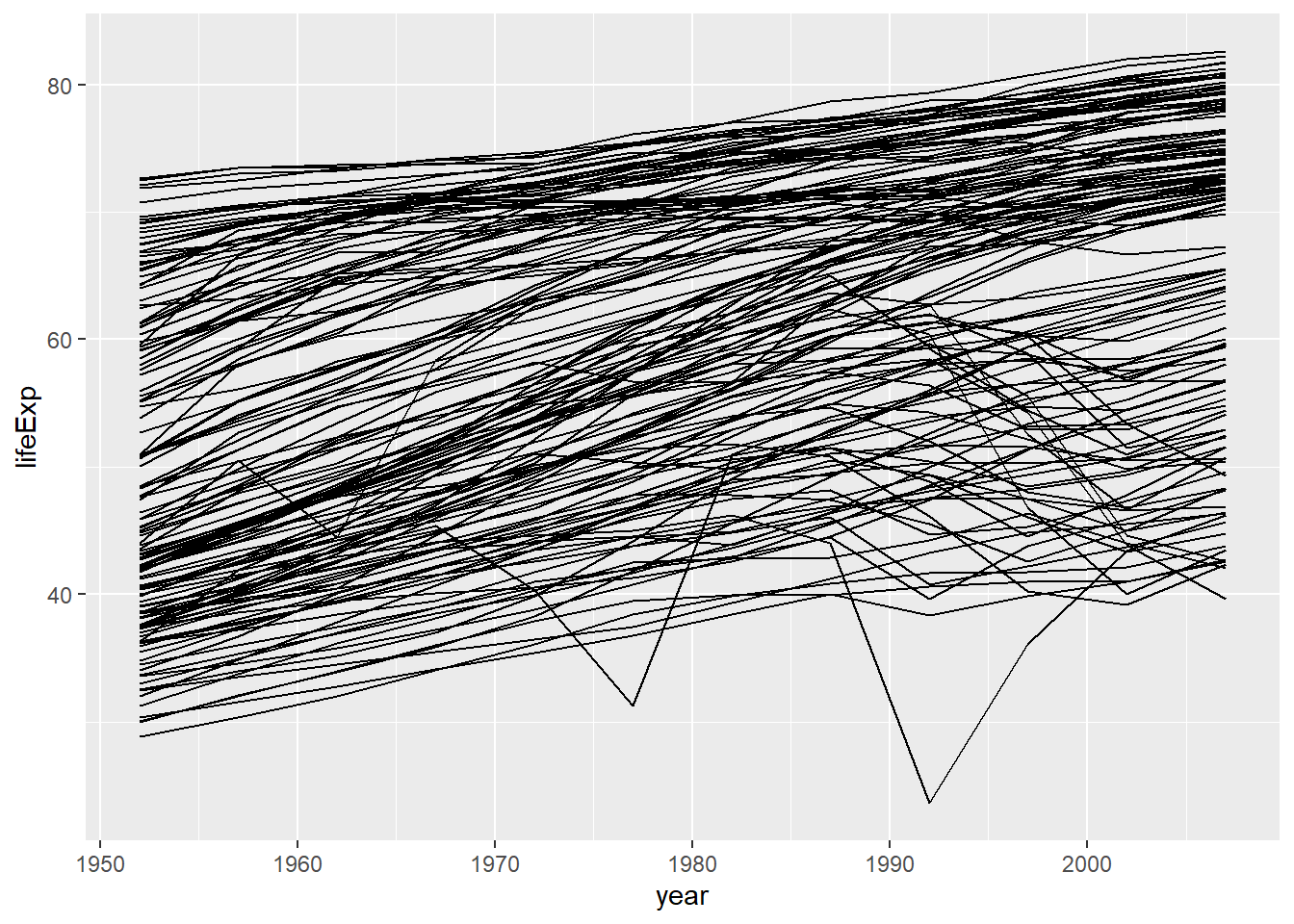
靠,这一团乱麻的东西是啥玩意。大概能看出预期寿命随着时间在增加,但仔细看的话有些国家不遵循这个趋势。怎样把他们分离出来呢?跟之前的模型处理一样。
Af <- gapminder %>% filter(country == "Afghanistan")

Af %>%
  ggplot(aes(year, lifeExp)) +
  geom_line() +
  ggtitle("Full data")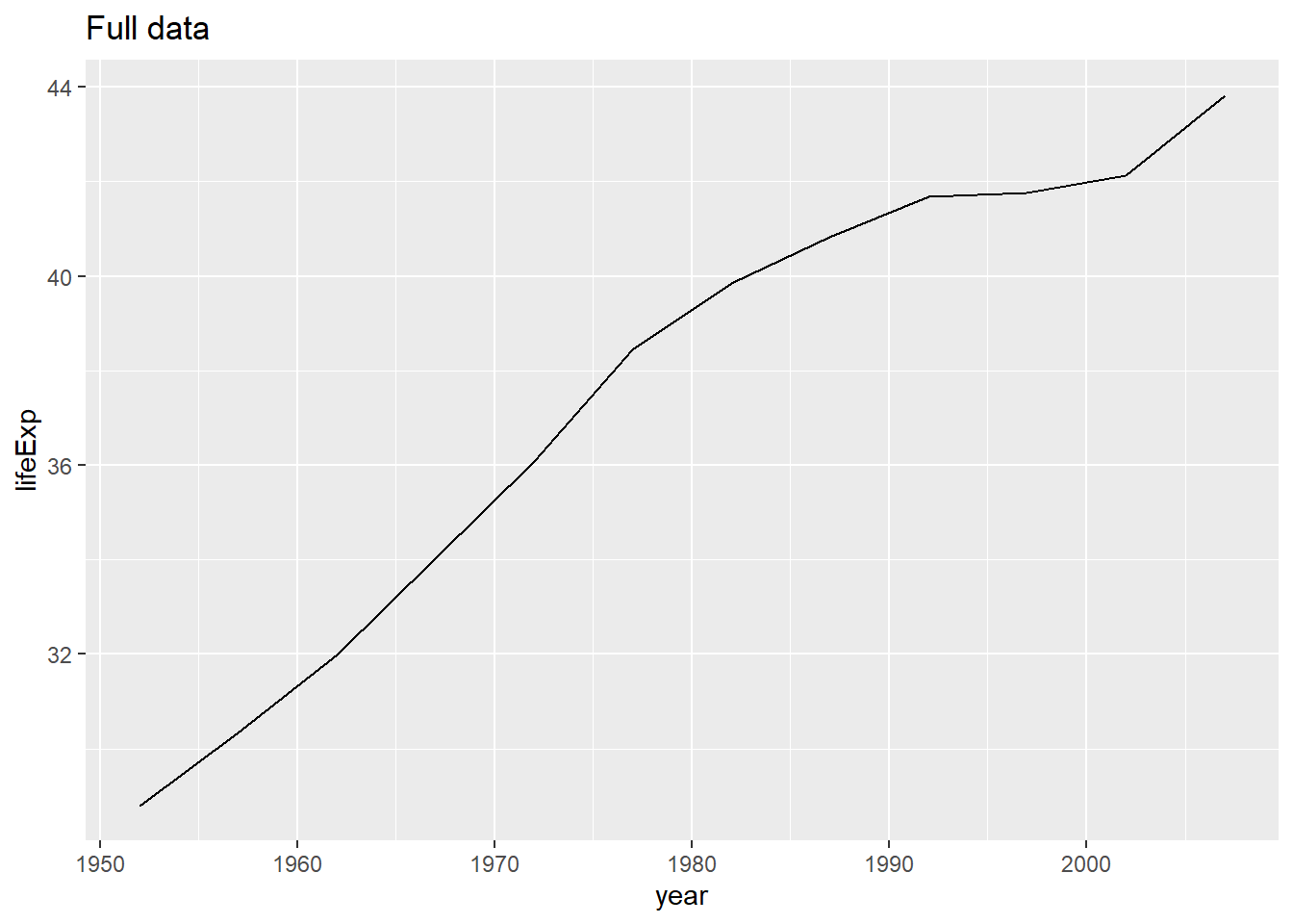
Af_model <- lm(lifeExp ~ year, data = Af)

Af %>%
  add_predictions(Af_model) %>%
  ggplot(aes(year, pred)) +
  geom_line() +
  ggtitle("Line trend")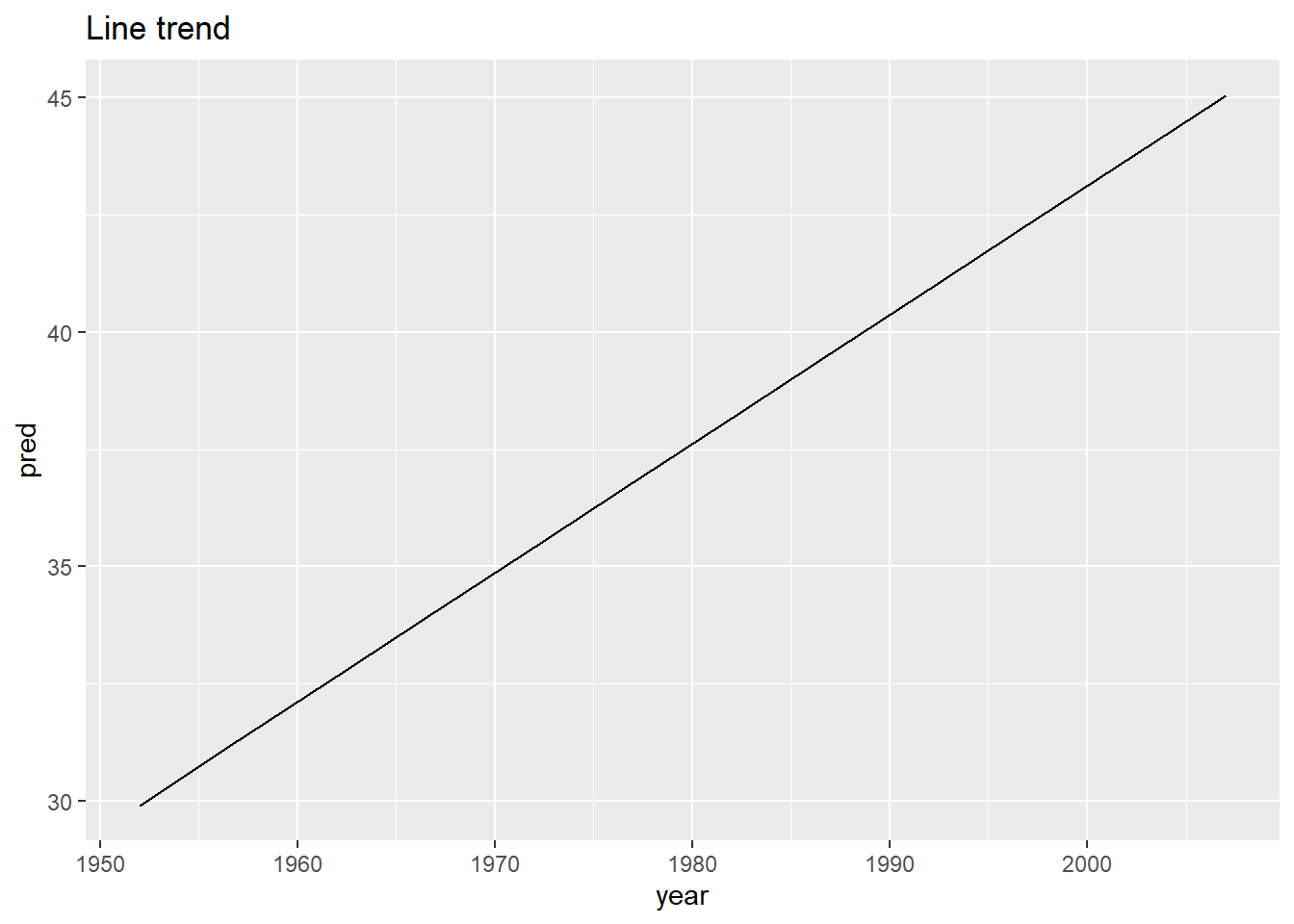
Af %>%
  add_residuals(Af_model) %>%
  ggplot(aes(year, resid)) +
  geom_point(size = 2, col = "blue") +
  geom_line() +
  geom_ref_line(h = 0) +
  ggtitle("Remaining pattern")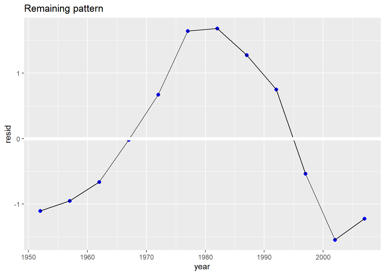
这么多国家难道要一个个弄?
5.2 聚合数据(nest data)
前面学过使用purrr::map()可以遍历列变量进行同样的操作。但这次需要对country变量的每一个类别建模,这需要使用**nested data fram,如下:
by_country <- gapminder %>%
  group_by(country, continent) %>%
  nest()
by_country
## # A tibble: 142 x 3
## # Groups: country, continent [142]
## country continent data
## <fct> <fct> <list>
## 1 Afghanistan Asia <tibble [12 x 4]>
## 2 Albania Europe <tibble [12 x 4]>
## 3 Algeria Africa <tibble [12 x 4]>
## 4 Angola Africa <tibble [12 x 4]>
## 5 Argentina Americas <tibble [12 x 4]>
## 6 Australia Oceania <tibble [12 x 4]>
## 7 Austria Europe <tibble [12 x 4]>
## 8 Bahrain Asia <tibble [12 x 4]>
## 9 Bangladesh Asia <tibble [12 x 4]>
## 10 Belgium Europe <tibble [12 x 4]>
## # ... with 132 more rows看看那缩成一坨的data列里面都是些什么,国家太多,我们看看第一个Afghanistan。
by_country$data[1]## [[1]]
## # A tibble: 12 x 4
## year lifeExp pop gdpPercap
## <int> <dbl> <int> <dbl>
## 1 1952 28.8 8425333 779.
## 2 1957 30.3 9240934 821.
## 3 1962 32.0 10267083 853.
## 4 1967 34.0 11537966 836.
## 5 1972 36.1 13079460 740.
## 6 1977 38.4 14880372 786.
## 7 1982 39.9 12881816 978.
## 8 1987 40.8 13867957 852.
## 9 1992 41.7 16317921 649.
## 10 1997 41.8 22227415 635.
## 11 2002 42.1 25268405 727.
## 12 2007 43.8 31889923 975.可以看数据的列表列中包含了1个国家的所有信息。
好了,现在我们定义一个建模的函数:
country_model <- function(df){
  lm(lifeExp ~ year, data = df)
}将建立的模型储存在原数据框的新的列model中:
by_country <-  by_country %>%
  mutate(model = map(data, ~ lm(lifeExp ~ year, data = .)))
现在可以随意筛选、排序数据获得你想要的数据:
by_country %>%
  filter(continent == "Asia")
## # A tibble: 33 x 4
## # Groups: country, continent [33]
## country continent data model
## <fct> <fct> <list> <list>
## 1 Afghanistan Asia <tibble [12 x 4]> <lm>
## 2 Bahrain Asia <tibble [12 x 4]> <lm>
## 3 Bangladesh Asia <tibble [12 x 4]> <lm>
## 4 Cambodia Asia <tibble [12 x 4]> <lm>
## 5 China Asia <tibble [12 x 4]> <lm>
## 6 Hong Kong, China Asia <tibble [12 x 4]> <lm>
## 7 India Asia <tibble [12 x 4]> <lm>
## 8 Indonesia Asia <tibble [12 x 4]> <lm>
## 9 Iran Asia <tibble [12 x 4]> <lm>
## 10 Iraq Asia <tibble [12 x 4]> <lm>
## # ... with 23 more rows5.3 展开Unnesting
现在有了142个数据框和142个模型,可以利用这些来计算残差,预测值等操作了:
by_country <- by_country %>%
  mutate(resids = map2(data, model, add_residuals),
         pred = map2(data, model, add_predictions))
by_country
## # A tibble: 142 x 6
## # Groups: country, continent [142]
## country continent data model resids pred
## <fct> <fct> <list> <list> <list> <list>
## 1 Afghanistan Asia <tibble [12 x 4]> <lm> <tibble [12 x 5]> <tibble [12~
## 2 Albania Europe <tibble [12 x 4]> <lm> <tibble [12 x 5]> <tibble [12~
## 3 Algeria Africa <tibble [12 x 4]> <lm> <tibble [12 x 5]> <tibble [12~
## 4 Angola Africa <tibble [12 x 4]> <lm> <tibble [12 x 5]> <tibble [12~
## 5 Argentina Americas <tibble [12 x 4]> <lm> <tibble [12 x 5]> <tibble [12~
## 6 Australia Oceania <tibble [12 x 4]> <lm> <tibble [12 x 5]> <tibble [12~
## 7 Austria Europe <tibble [12 x 4]> <lm> <tibble [12 x 5]> <tibble [12~
## 8 Bahrain Asia <tibble [12 x 4]> <lm> <tibble [12 x 5]> <tibble [12~
## 9 Bangladesh Asia <tibble [12 x 4]> <lm> <tibble [12 x 5]> <tibble [12~
## 10 Belgium Europe <tibble [12 x 4]> <lm> <tibble [12 x 5]> <tibble [12~
## # ... with 132 more rows但是列表列怎么画图呢?先不纠结这个问题,先把所有的nest用unnest展开看看
resids <-  by_country %>% unnest(resids)
resids
## # A tibble: 1,704 x 10
## # Groups: country, continent [142]
## country continent data model year lifeExp pop gdpPercap resid pred
## <fct> <fct> <list> <lis> <int> <dbl> <int> <dbl> <dbl> <list>
## 1 Afghani~ Asia <tibb~ <lm> 1952 28.8 8.43e6 779. -1.11 <tibb~
## 2 Afghani~ Asia <tibb~ <lm> 1957 30.3 9.24e6 821. -0.952 <tibb~
## 3 Afghani~ Asia <tibb~ <lm> 1962 32.0 1.03e7 853. -0.664 <tibb~
## 4 Afghani~ Asia <tibb~ <lm> 1967 34.0 1.15e7 836. -0.0172 <tibb~
## 5 Afghani~ Asia <tibb~ <lm> 1972 36.1 1.31e7 740. 0.674 <tibb~
## 6 Afghani~ Asia <tibb~ <lm> 1977 38.4 1.49e7 786. 1.65 <tibb~
## 7 Afghani~ Asia <tibb~ <lm> 1982 39.9 1.29e7 978. 1.69 <tibb~
## 8 Afghani~ Asia <tibb~ <lm> 1987 40.8 1.39e7 852. 1.28 <tibb~
## 9 Afghani~ Asia <tibb~ <lm> 1992 41.7 1.63e7 649. 0.754 <tibb~
## 10 Afghani~ Asia <tibb~ <lm> 1997 41.8 2.22e7 635. -0.534 <tibb~
## # ... with 1,694 more rows现在看到数据按照年份展开了,可以画图看看
resids %>%
  ggplot(aes(year, resid)) +
  geom_line(aes(group = country, alpha = 1/3)) +
  geom_smooth(se = F)
## `geom_smooth()` using method = 'gam' and formula 'y ~ s(x, bs = "cs")'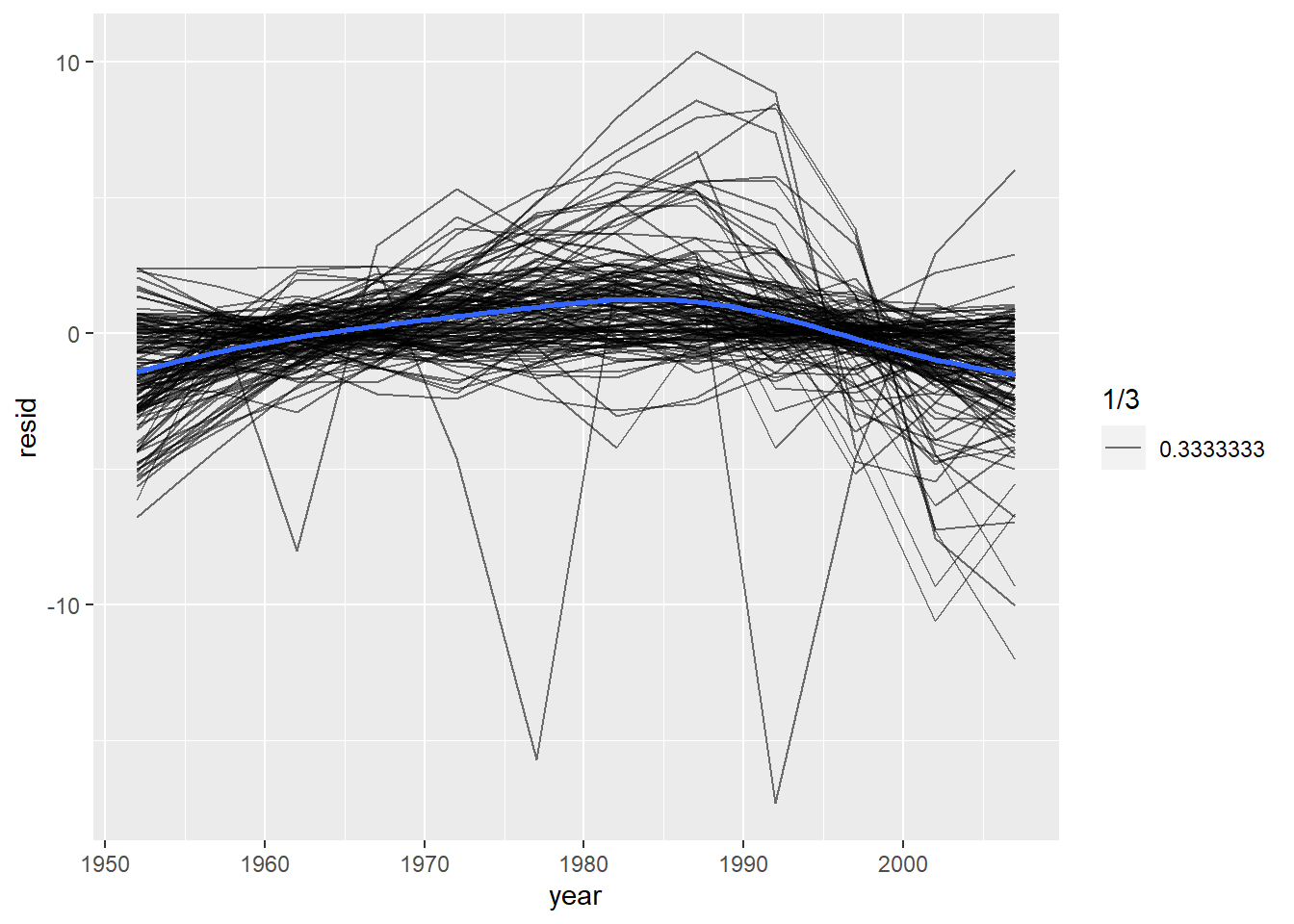 按照大洲分面绘制:
resids %>%
ggplot(aes(year, resid)) +
geom_line(aes(group = country, alpha = 1/3)) +
facet_wrap(~ continent)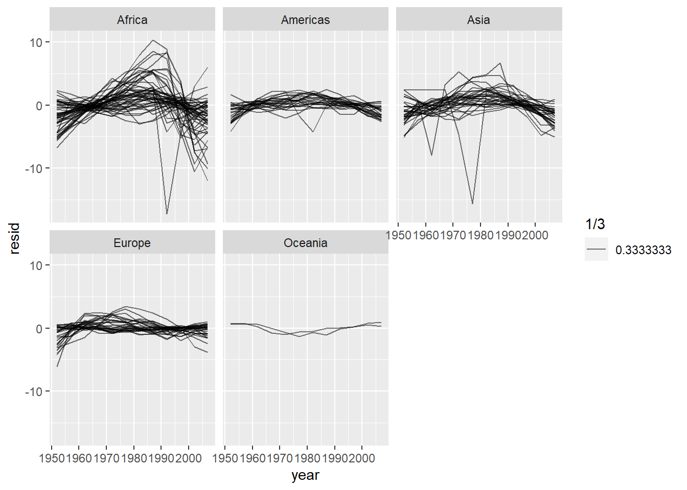 看起来好像有些轻微的趋势被忽略了,而且非洲的模型看起来有一些较大的残差。
5.4 模型质量
除了看模型残差分布外,还可以使用其他的一些统计指标来衡量模型质量。broom包中的glance可以提取衡量模型质量的指标。
broom::glance(Af_model)## # A tibble: 1 x 12
## r.squared adj.r.squared sigma statistic p.value df logLik AIC BIC
## <dbl> <dbl> <dbl> <dbl> <dbl> <dbl> <dbl> <dbl> <dbl>
## 1 0.948 0.942 1.22 181. 0.0000000984 1 -18.3 42.7 44.1
## # ... with 3 more variables: deviance <dbl>, df.residual <int>, nobs <int>使用mutate()和unnest()创建一个数据框:
by_country %>%
  mutate(glance = map(model, broom::glance)) %>%
  unnest(glance)
## # A tibble: 142 x 18
## # Groups: country, continent [142]
## country continent data model resids pred r.squared adj.r.squared sigma
## <fct> <fct> <list> <lis> <list> <lis> <dbl> <dbl> <dbl>
## 1 Afghanistan Asia <tibb~ <lm> <tibb~ <tib~ 0.948 0.942 1.22
## 2 Albania Europe <tibb~ <lm> <tibb~ <tib~ 0.911 0.902 1.98
## 3 Algeria Africa <tibb~ <lm> <tibb~ <tib~ 0.985 0.984 1.32
## 4 Angola Africa <tibb~ <lm> <tibb~ <tib~ 0.888 0.877 1.41
## 5 Argentina Americas <tibb~ <lm> <tibb~ <tib~ 0.996 0.995 0.292
## 6 Australia Oceania <tibb~ <lm> <tibb~ <tib~ 0.980 0.978 0.621
## 7 Austria Europe <tibb~ <lm> <tibb~ <tib~ 0.992 0.991 0.407
## 8 Bahrain Asia <tibb~ <lm> <tibb~ <tib~ 0.967 0.963 1.64
## 9 Bangladesh Asia <tibb~ <lm> <tibb~ <tib~ 0.989 0.988 0.977
## 10 Belgium Europe <tibb~ <lm> <tibb~ <tib~ 0.995 0.994 0.293
## # ... with 132 more rows, and 9 more variables: statistic <dbl>, p.value <dbl>,
## # df <dbl>, logLik <dbl>, AIC <dbl>, BIC <dbl>, deviance <dbl>,
## # df.residual <int>, nobs <int>添加.drop = T:
glance <-  by_country %>%
  mutate(glance = map(model, broom::glance)) %>%
  unnest(glance, .drop = T)
## Warning: The `.drop` argument of `unnest()` is deprecated as of tidyr 1.0.0.
## All list-columns are now preserved.
## This warning is displayed once every 8 hours.
## Call `lifecycle::last_lifecycle_warnings()` to see where this warning was generated.glance## # A tibble: 142 x 18
## # Groups: country, continent [142]
## country continent data model resids pred r.squared adj.r.squared sigma
## <fct> <fct> <list> <lis> <list> <lis> <dbl> <dbl> <dbl>
## 1 Afghanistan Asia <tibb~ <lm> <tibb~ <tib~ 0.948 0.942 1.22
## 2 Albania Europe <tibb~ <lm> <tibb~ <tib~ 0.911 0.902 1.98
## 3 Algeria Africa <tibb~ <lm> <tibb~ <tib~ 0.985 0.984 1.32
## 4 Angola Africa <tibb~ <lm> <tibb~ <tib~ 0.888 0.877 1.41
## 5 Argentina Americas <tibb~ <lm> <tibb~ <tib~ 0.996 0.995 0.292
## 6 Australia Oceania <tibb~ <lm> <tibb~ <tib~ 0.980 0.978 0.621
## 7 Austria Europe <tibb~ <lm> <tibb~ <tib~ 0.992 0.991 0.407
## 8 Bahrain Asia <tibb~ <lm> <tibb~ <tib~ 0.967 0.963 1.64
## 9 Bangladesh Asia <tibb~ <lm> <tibb~ <tib~ 0.989 0.988 0.977
## 10 Belgium Europe <tibb~ <lm> <tibb~ <tib~ 0.995 0.994 0.293
## # ... with 132 more rows, and 9 more variables: statistic <dbl>, p.value <dbl>,
## # df <dbl>, logLik <dbl>, AIC <dbl>, BIC <dbl>, deviance <dbl>,
## # df.residual <int>, nobs <int>筛选一下拟合差的模型:
glance %>%
  filter(r.squared < 0.25)
## # A tibble: 6 x 18
## # Groups: country, continent [6]
## country continent data model resids pred r.squared adj.r.squared sigma
## <fct> <fct> <list> <lis> <list> <list> <dbl> <dbl> <dbl>
## 1 Botswana Africa <tibbl~ <lm> <tibbl~ <tibb~ 0.0340 -0.0626 6.11
## 2 Lesotho Africa <tibbl~ <lm> <tibbl~ <tibb~ 0.0849 -0.00666 5.93
## 3 Rwanda Africa <tibbl~ <lm> <tibbl~ <tibb~ 0.0172 -0.0811 6.56
## 4 Swaziland Africa <tibbl~ <lm> <tibbl~ <tibb~ 0.0682 -0.0250 6.64
## 5 Zambia Africa <tibbl~ <lm> <tibbl~ <tibb~ 0.0598 -0.0342 4.53
## 6 Zimbabwe Africa <tibbl~ <lm> <tibbl~ <tibb~ 0.0562 -0.0381 7.21
## # ... with 9 more variables: statistic <dbl>, p.value <dbl>, df <dbl>,
## # logLik <dbl>, AIC <dbl>, BIC <dbl>, deviance <dbl>, df.residual <int>,
## # nobs <int>拟合差的模型看起来好像都是在非洲:
glance %>%
ggplot(aes(continent, r.squared)) +
geom_jitter()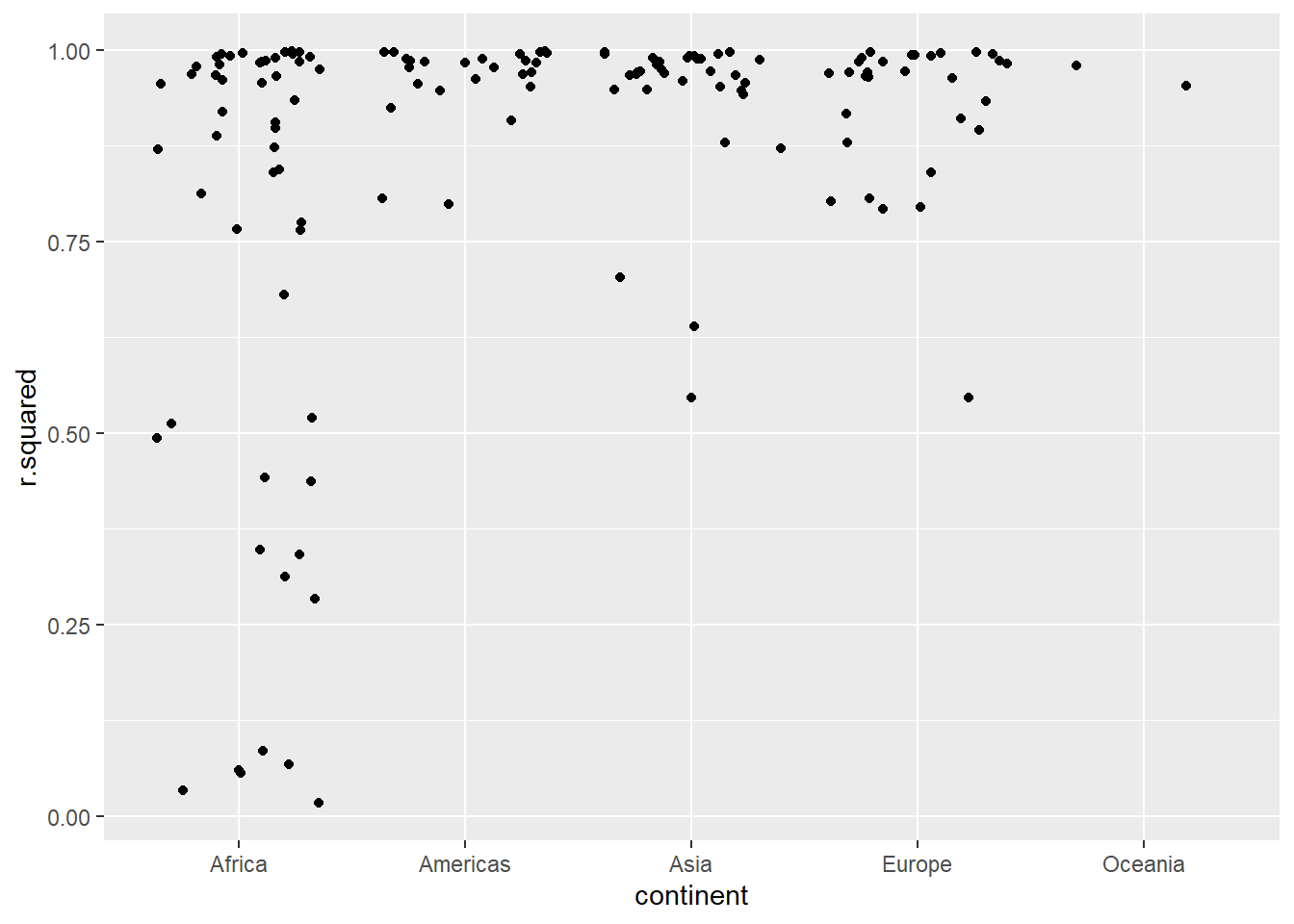 把拟合差的国家原始数据筛选出来:
bad_fit <- filter(glance, r.squared < 0.25)
gapminder %>%
semi_join(bad_fit, by = "country") %>%
ggplot(aes(year, lifeExp, colour = country)) +
geom_line()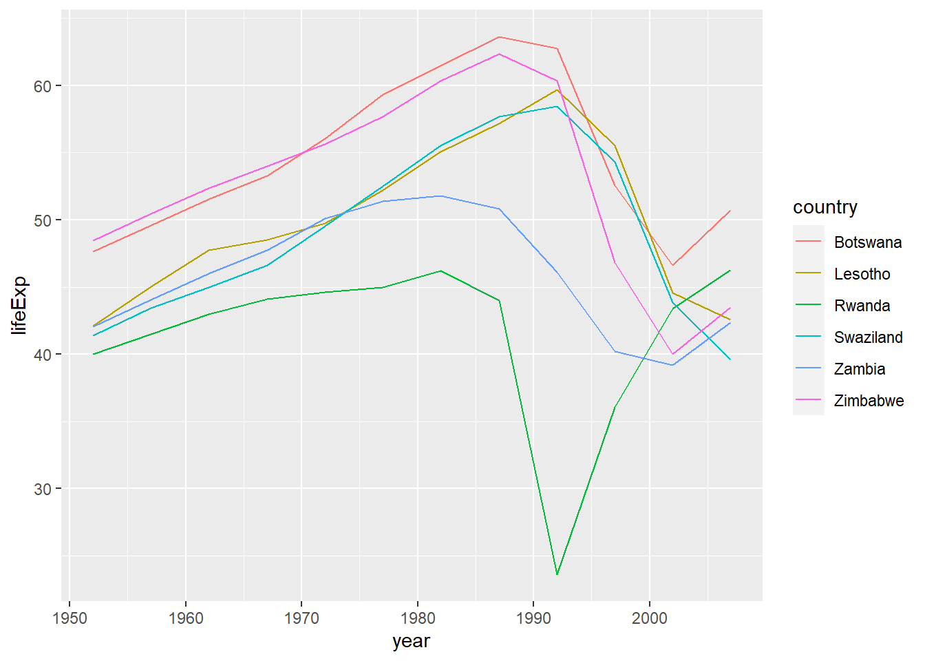 ### 练习题:
- 对于整体趋势来说,线性关系过于简单,添加多项式是否更合适。但怎么解释二次方的系数呢?
答:使用poly(x, degree = )可以生成变量的正交多项式来进行多项式拟合
country_model2 <-  function(df) {
  lm(lifeExp ~ poly(year - median(2), 2), data = df)
}

by_country <- by_country %>%
  mutate(model = map(data, country_model2))
by_country
## # A tibble: 142 x 6
## # Groups: country, continent [142]
## country continent data model resids pred
## <fct> <fct> <list> <list> <list> <list>
## 1 Afghanistan Asia <tibble [12 x 4]> <lm> <tibble [12 x 5]> <tibble [12~
## 2 Albania Europe <tibble [12 x 4]> <lm> <tibble [12 x 5]> <tibble [12~
## 3 Algeria Africa <tibble [12 x 4]> <lm> <tibble [12 x 5]> <tibble [12~
## 4 Angola Africa <tibble [12 x 4]> <lm> <tibble [12 x 5]> <tibble [12~
## 5 Argentina Americas <tibble [12 x 4]> <lm> <tibble [12 x 5]> <tibble [12~
## 6 Australia Oceania <tibble [12 x 4]> <lm> <tibble [12 x 5]> <tibble [12~
## 7 Austria Europe <tibble [12 x 4]> <lm> <tibble [12 x 5]> <tibble [12~
## 8 Bahrain Asia <tibble [12 x 4]> <lm> <tibble [12 x 5]> <tibble [12~
## 9 Bangladesh Asia <tibble [12 x 4]> <lm> <tibble [12 x 5]> <tibble [12~
## 10 Belgium Europe <tibble [12 x 4]> <lm> <tibble [12 x 5]> <tibble [12~
## # ... with 132 more rowsby_country <- by_country %>%
mutate(resids = map2(data, model, add_residuals))
by_country## # A tibble: 142 x 6
## # Groups: country, continent [142]
## country continent data model resids pred
## <fct> <fct> <list> <list> <list> <list>
## 1 Afghanistan Asia <tibble [12 x 4]> <lm> <tibble [12 x 5]> <tibble [12~
## 2 Albania Europe <tibble [12 x 4]> <lm> <tibble [12 x 5]> <tibble [12~
## 3 Algeria Africa <tibble [12 x 4]> <lm> <tibble [12 x 5]> <tibble [12~
## 4 Angola Africa <tibble [12 x 4]> <lm> <tibble [12 x 5]> <tibble [12~
## 5 Argentina Americas <tibble [12 x 4]> <lm> <tibble [12 x 5]> <tibble [12~
## 6 Australia Oceania <tibble [12 x 4]> <lm> <tibble [12 x 5]> <tibble [12~
## 7 Austria Europe <tibble [12 x 4]> <lm> <tibble [12 x 5]> <tibble [12~
## 8 Bahrain Asia <tibble [12 x 4]> <lm> <tibble [12 x 5]> <tibble [12~
## 9 Bangladesh Asia <tibble [12 x 4]> <lm> <tibble [12 x 5]> <tibble [12~
## 10 Belgium Europe <tibble [12 x 4]> <lm> <tibble [12 x 5]> <tibble [12~
## # ... with 132 more rowsunnest(by_country, resids) %>%
ggplot(aes(year, resid)) +
geom_point(aes(group = country)) +
geom_smooth() +
geom_ref_line(h = 0)## `geom_smooth()` using method = 'gam' and formula 'y ~ s(x, bs = "cs")'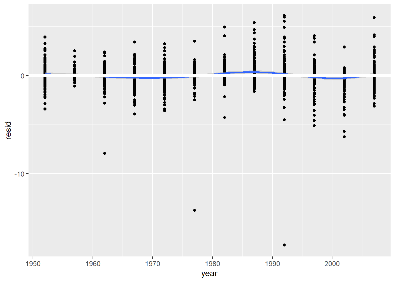
by_country %>%
mutate(glance = map(model, broom::glance)) %>%
unnest(glance, .drop = T) %>%
ggplot(aes(continent, r.squared)) +
geom_jitter()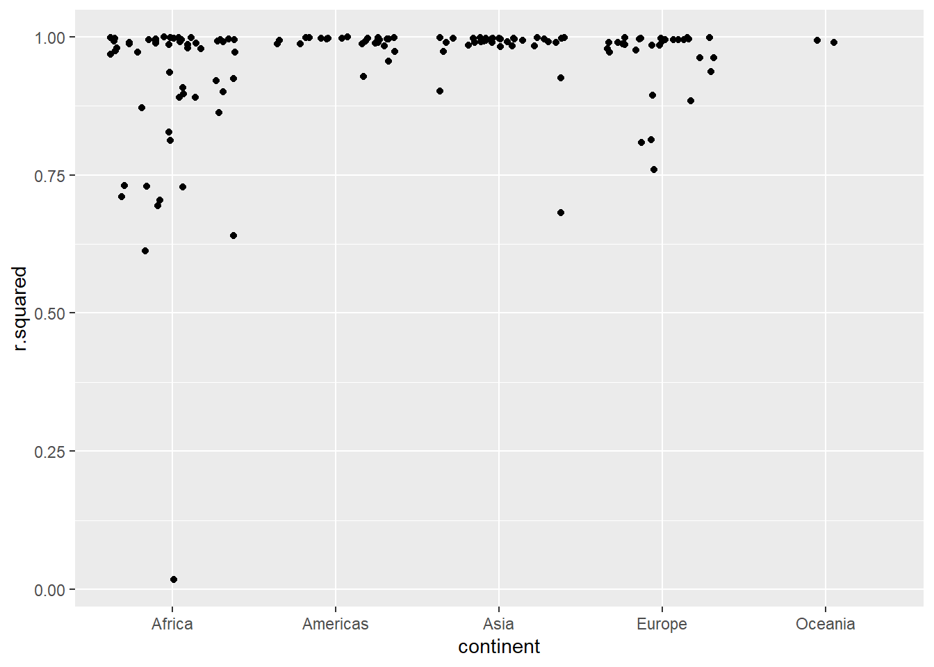 `
`