Chapter 5 Big Data Applications
Big data has revolutionized the way the financial industry operates by providing vast amounts of information that can be analyzed to identify patterns and trends, make predictions, and inform business decisions. In finance, big data is generated from a variety of sources, including market data, customer data, social media, and news feeds. The ability to collect and analyze this data has opened up new opportunities for financial institutions to improve customer experiences, optimize business processes, and make more informed investment decisions.
This section will elaborate on structuring data science projects, introduce different concepts of machine learning and regression techniques.
5.1 Structuring Projects
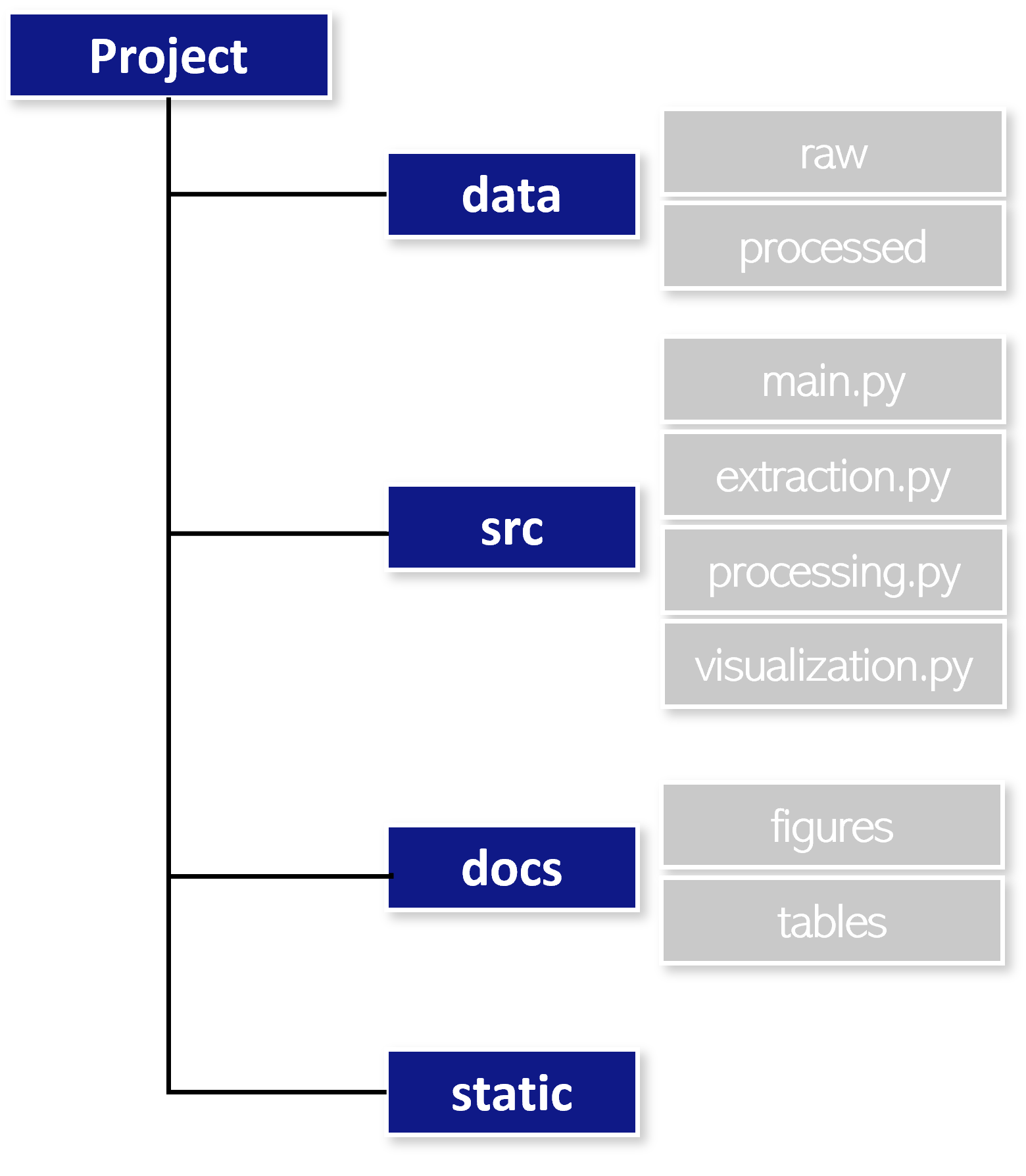
The structuring of data science projects is not absolute and can be subject to own personal preferences. If the project contains a vast amount of code, single code snippets should be divivded by functionality to be placed into separate files keeping the single coding files clean and concise. The folder that contains the source code is by convention called src. It contains all relevant scripts. In order to keep track of project progression and capture findings you might want to initialize a docs folder, indicating project documentation. The documentation folder can contain subfolders which keep figures, tables and verbal explaination of the preliminary findings. Finally, the folder data contains relevant datasets in raw and processed form for the analysis. Static objects, can be put into a static folder.
They might also contain a virtual environment Virtual environments are commonly used in Python development to isolate projects and ensure that each project has access to the correct versions of libraries and dependencies. A virtual environment is a self-contained directory that contains a specific version of Python and its associated libraries and dependencies. It allows multiple versions of Python and its dependencies to coexist on the same system without interfering with each other. This is especially useful to reproduce output on another machine or to share a project with others.
5.2 Model Development
There are many algorithms and methods available that you may want to choose for your problem — however, it is often wise to start with a simple method and then reiterate. It also involves the determination of relevant input variables as in the term of data engineering. Complex machine learning often obtain an advanced degree of precision, however they are perceived as Black Boxes that create desirable output.
We therefore think about a suitable characterization of the data generating process. The data generating process is the underlying mechanism that produces the observed data in a statistical or machine learning analysis. It is a model that describes how the data was generated from the underlying population or system that the data represents. Understanding the data generating process is important in statistical and machine learning analysis, as it allows researchers to make assumptions about the behavior of the system and to choose appropriate models and estimation methods. We tend to investigate (i) relevant input variables and (ii) the functional form of the data generating process.
Generally, we differentiate between three distinguishable machine learning paradigms. The most suitable approach oftentimes depends on the data and problem at hand.
| Supervised Learning | Modelling with labelled data. The response variable is apparent and its realizations are available. Since the variable is numeric the model will be used to infer about classification and regression analysis. The algorithm is given a set of inputs and corresponding outputs and learns to map the inputs to the correct outputs. The goal of supervised learning is to learn a function that can predict outputs for new, unseen inputs. |
| Unsupervised Learning | No response variable is given. The model is used to create transparency about unobserved patterns within the data. Unsupervised learning is a type of machine learning where the algorithm learns to identify patterns or relationships in data without any labeled examples. In unsupervised learning, the algorithm is given a set of inputs and no corresponding outputs, and it learns to find structure or regularities in the data. |
| Reinforcement Learning | The agent (model) interacts and determines suitable actions after the model has been proposed. It deals with sequential decision making, therefore the output depends on the state of the current input and the next input depends on the preceding output. Reinforcement learning is a subfield of machine learning that involves training an agent to learn how to make decisions based on the environment it is in. In reinforcement learning, an agent interacts with an environment by taking actions and receiving rewards or penalties for those actions. The agent’s goal is to learn a policy, or a mapping from states to actions, that maximizes its cumulative reward over time. |
| Regression | Regression is used to predict a continuous output variable based on input features. It is used when the output variable is numerical in nature. |
| Classification | Classification is used to predict a categorical output variable based on input features. It is used when the output variable is discrete in nature. |
| Support Vector Machines | Support Vector Machines is a type of supervised learning algorithm used for both regression and classification problems. It is used to find the best boundary between different classes of data points. |
| Decision Trees | Decision trees are a type of supervised learning algorithm used for classification and regression problems. It is used to build a tree-like model of decisions and their possible consequences. |
| Random Forest | Random Forest is an ensemble learning method used for classification, regression, and other tasks. It involves building multiple decision trees and combining their predictions to improve accuracy. |
| Naive Bayes | Naive Bayes is a probabilistic algorithm used for classification problems. It is based on Bayes’ theorem and assumes that the input features are independent of each other. |
| Neural Networks | Neural Networks are a type of machine learning algorithm inspired by the structure and function of the human brain. They are used for both regression and classification problems and have been shown to be highly effective in a variety of applications. |
Unsupervised Learning
We will employ a clustering algorithm by using a multitude of attributes for the sample of stocks.
We anonymize the trade data by removing the symbol column to allow the algorithm to find the optimal number of groups within the sample.
Since we have been working with the data previously, we already know the answer will be two.
We will work with data from AMZN, PEP on the 2022-02-01.
We extract the data, compute logarithmic returns and volatility.
We obtain the following return structure throughout the trading day
# Returns throughout trading day
ggplot() + \
    geom_point(trades_grouped, aes(x="parttime_trade_rounded",
                                   y="return",
                                   group="sym",
                                   color="sym"), alpha=0.2) + \
    geom_hline(yintercept=0) + \
    ylim(-10**-3, 10**-3) + \
    xlab("Time") + \
    ylab("Logarithmic Return") + \
    scale_x_datetime(date_labels = "%H:%M") + \
    scale_color_manual([custom_blue, custom_red]) + \
    theme_custom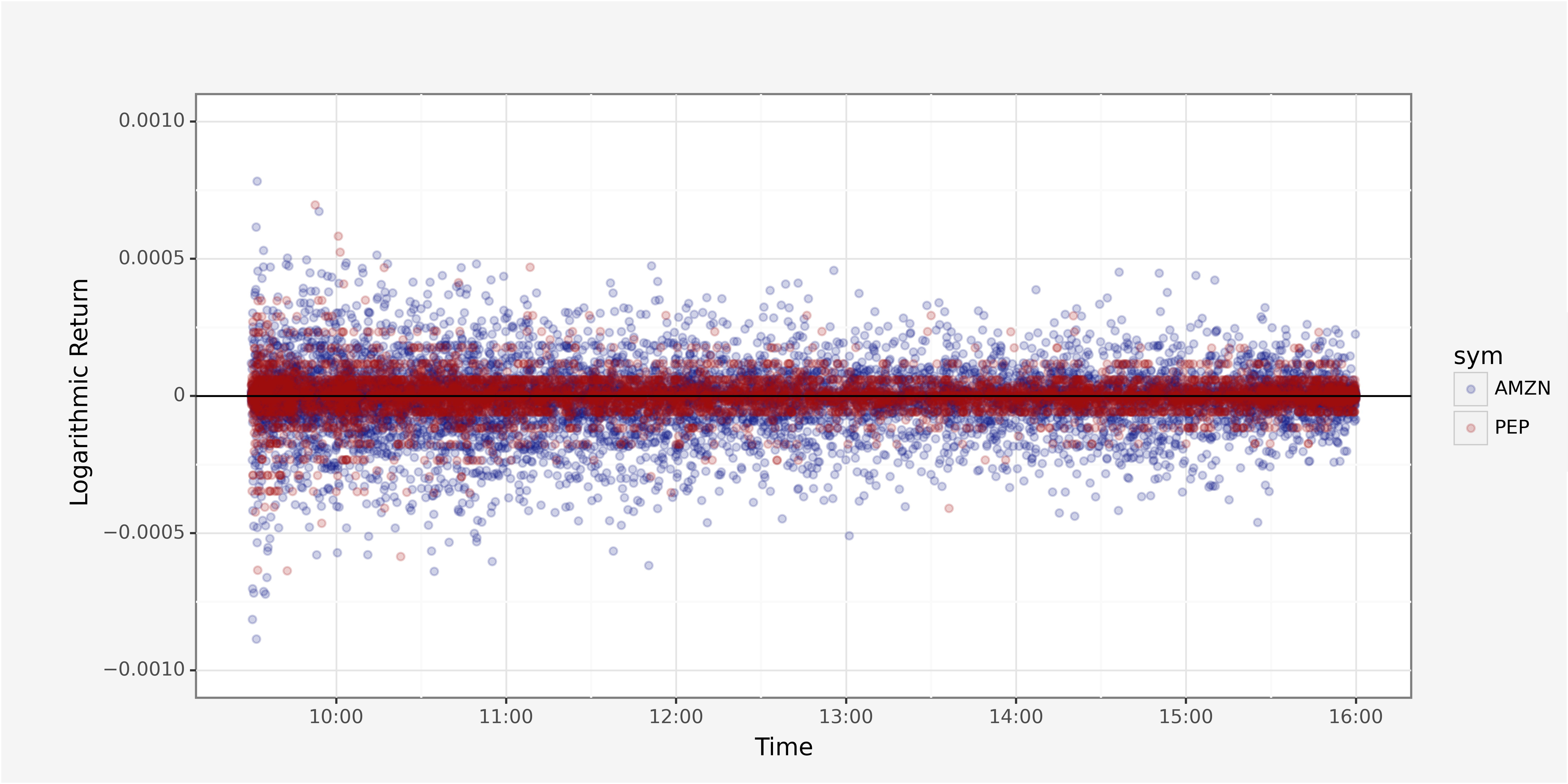
And volatility as sum of squared returns per trading second.
# Unaggregated volatility plot
ggplot() + \
    geom_point(trades_grouped, aes(x="parttime_trade_rounded",
                                   y="volatility",
                                   group="sym",
                                   color="sym"), alpha=0.1) + \
    geom_hline(yintercept=0) + \
    ylim(0, 0.0000025) + \
    xlab("Time") + \
    ylab("Volatility") + \
    scale_x_datetime(date_labels = "%H:%M") + \
    scale_color_manual([custom_blue, custom_red]) + \
    theme_custom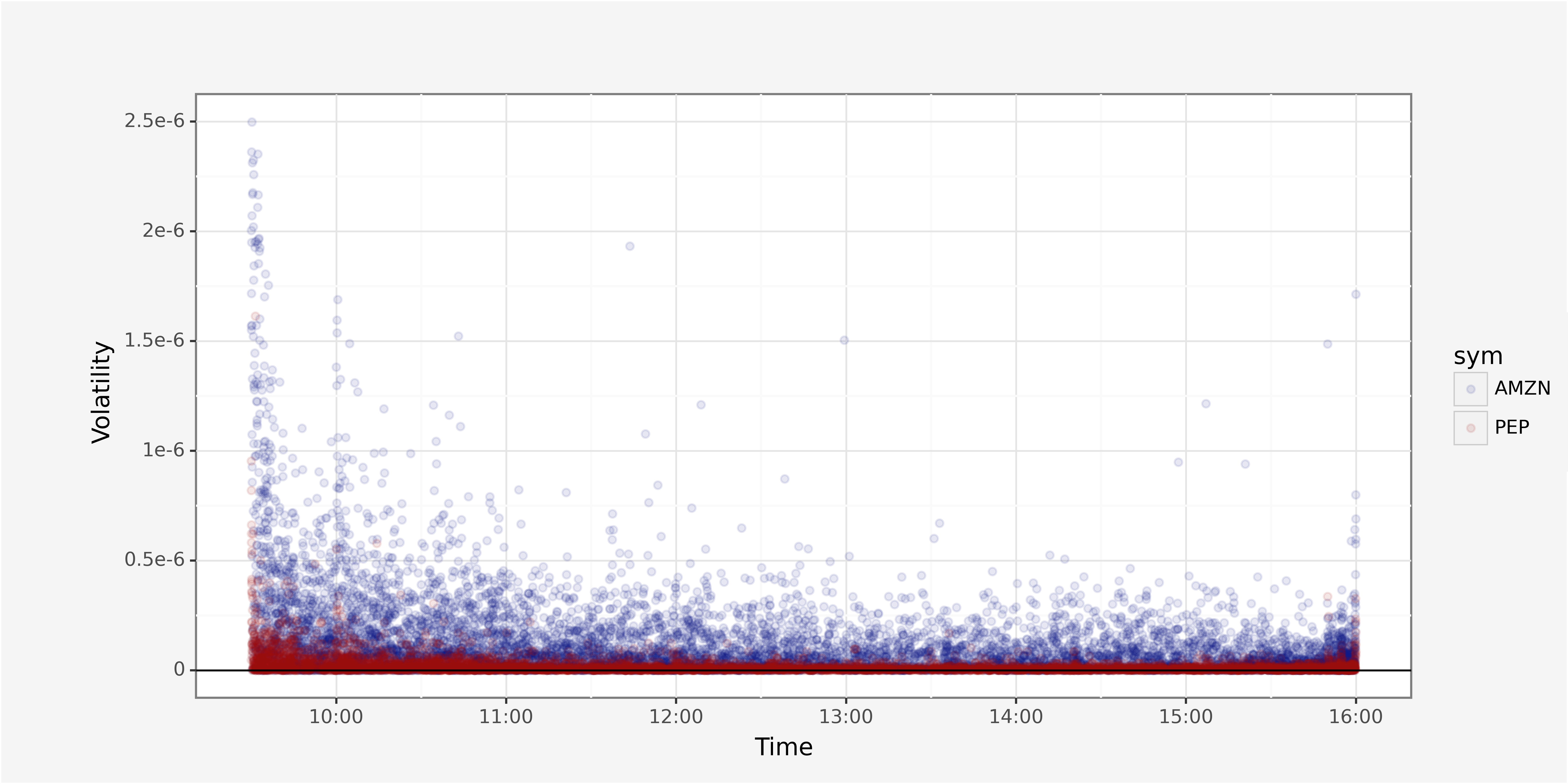
The aggregation on minute intervals allows to plot a cleaner version of intraday volatility.
We can clearly see that the volatility follows a function that seems to have hyperbolic decay of the form
\(\sigma_t = \frac{1}{\alpha \times t + 1} + c \quad t \in \quad [0,390]\)
with \(t\) indicating the minute after exchange opening time.
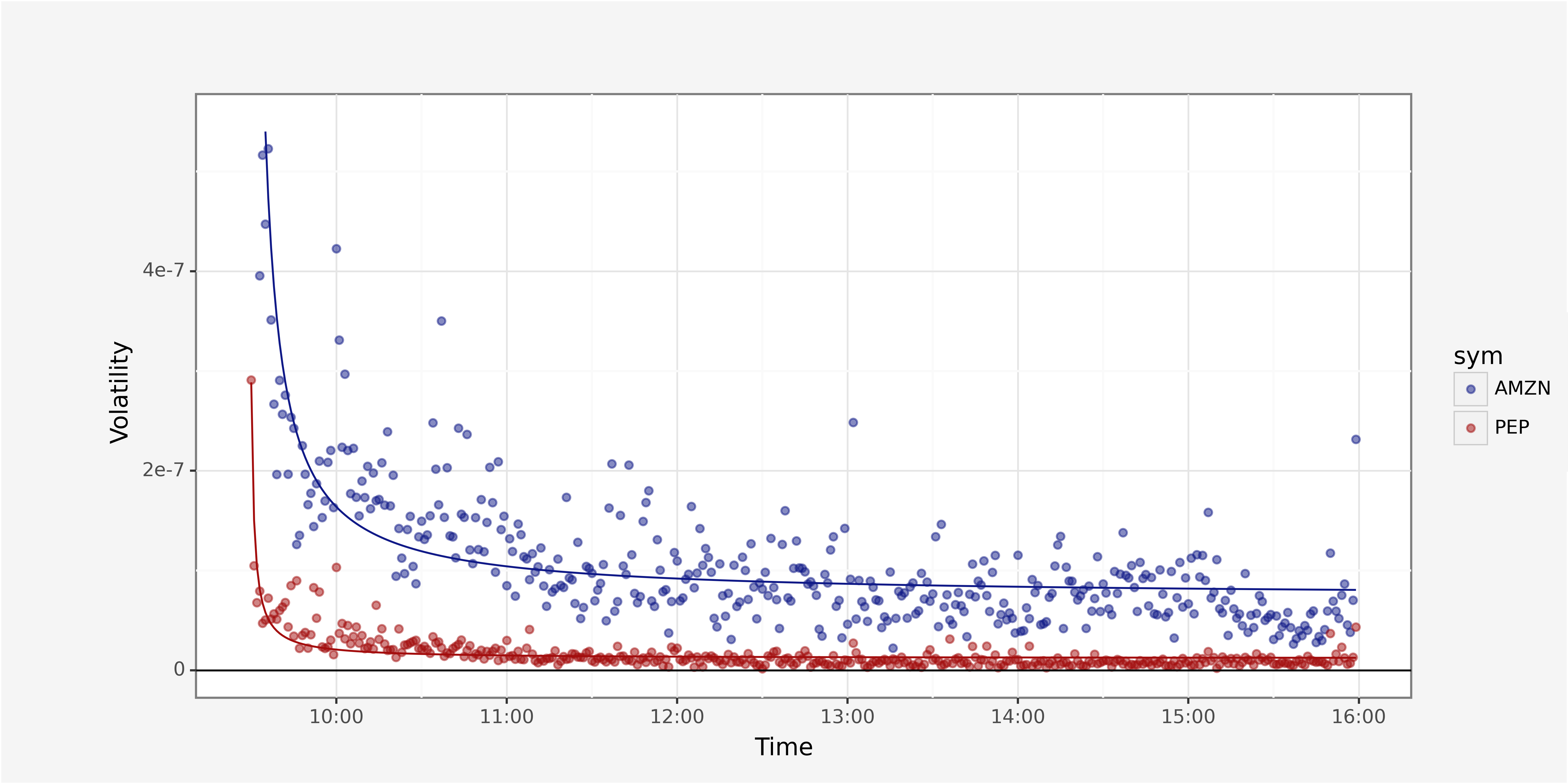
We now want to use a supervised learning algorithm to identify the best coefficient for \(\alpha\) and \(c\) for each of the stocks. This process is called hyperparameter tuning. There is a set of algorithms to obtain the optimal coefficients, such as grid search, random search, informed search.
An optimization Algorithm
In order to remove the term Black Box we want to look at the steps taken to identify optimal parameter values within a model.
Given a function \(f(x,\theta)\) that models a set of \(n\) data points, with \(\theta\) being the parameter vector to be estimated, the Levenberg-Marquardt algorithm aims to minimize the sum of squared residuals as
\(S(\theta) = \sum_{i=1}^n (y_i - f(x_i, \theta))^2\)
The algorithm iteratively updates the parameter vector \(\theta\) until it converges to a minimum of \(S(\theta)\). The Levenberg-Marquardt algorithm follows the steps
- Choose an initial value of the damping parameter \(\lambda\) and an initial estimate of \(\theta\).
- Compute the Jacobian matrix \(J\) of the model function \(f(x,\theta)\) at the current estimate of \(\theta\).
- Compute the residual vector \(r = (y - f(x, \theta))\).
- Compute the approximation to the Hessian matrix \(H\) using the Jacobian matrix and the damping parameter:
\(H \approx J^T J + \lambda I\)
- Solve the system of equations
\((J^T J + \lambda I) \Delta \theta = J^T r\)
for the parameter update \(\Delta \theta\).
- Compute the proposed new parameter vector as
\(\theta^* = \theta + \Delta \theta\)
- Compute the new residual vector \(r^* = (y - f(x, \theta^*))^2\).
- If the new sum of squared residuals \(S(\theta^*)\) is smaller than the current sum of squared residuals \(S(\theta)\), accept the proposed new parameter vector and decrease the damping parameter: \(\lambda \leftarrow \lambda / 10\). If the new sum of squared residuals \(S(\theta^*)\) is larger than the current sum of squared residuals \(S(\theta)\), reject the proposed new parameter vector and increase the damping parameter: \(\lambda \leftarrow \lambda * 10\).
- Iterate steps until the sum of squared residuals converges to a minimum.
In Python, this algorithm is what the function curve_fit does.
# Import modules
from scipy.optimize import curve_fit

# Define objective function
def objective(x, a, b):
    return (1 / (a*x+ 1)) + b

# Extract relevant values
x_values = list(range(1, len(minute_data.query("sym == 'AMZN'"))+1))
y_values = list(minute_data.query("sym == 'AMZN'").sort_values("parttime_trade_minute")["volatility"])

# Optimize curve parameters
popt_amzn, _ = curve_fit(objective, x_values, y_values, maxfev=10000)

# Compute values based on optimal curve parameters
volatility_amzn = pd.DataFrame(x_values, columns =["index"])
volatility_amzn["volatility"] = volatility_amzn.apply(lambda x: objective(x, popt_amzn[0], popt_amzn[1]))
volatility_amzn["parttime_trade_minute"] = minute_data.query("sym == 'AMZN'")["parttime_trade_minute"]
volatility_amzn.head(10)
We obtain the functional fit with the coefficients
# Returns versus Volatility
ggplot() + \
    geom_point(minute_data, aes(x="parttime_trade_minute", y="volatility", group="sym", color="sym"), alpha=0.5) + \
    geom_line(volatility_amzn, aes(x="parttime_trade_minute", y="volatility"), color=custom_blue) + \
    geom_line(volatility_pep, aes(x="parttime_trade_minute", y="volatility"), color=custom_red) + \
    geom_hline(yintercept=0) + \
    ylim(0, vola_threshold) + \
    xlab("Time") + \
    ylab("Volatility") + \
    scale_x_datetime(date_labels = "%H:%M") + \
    scale_color_manual([custom_blue, custom_red]) + \
    theme_custom
Hierarchical Clustering
Hierarchical clustering is a method of clustering that builds a hierarchy of clusters using a bottom-up or top-down approach.
This section will be extended
5.3 Model Evaluation
Model evaluation is the process of assessing the performance of a predictive model on a given dataset. The goal of model evaluation is to determine how well the model can adapt to new, unseen data and to identify potential issues with the model that need to be addressed.
In machine learning, there are several commonly used metrics for evaluating the performance of a model, depending on the nature of the problem being solved.
5.3.1 Bias and Variance
Bias and variance are important concepts to consider when training a model because they are key factors that influence the ability of the model to adapt to new data.
Bias refers to the degree to which a model’s predictions differ from the true values of the target variable, and is therefore only inherent to the model.
\(Bias_i = y_i - \hat{y}\)
A model with high bias tends to oversimplify the problem and may underfit the data, failing to capture important patterns in the data. In contrast, a model with low bias may be more complex and better able to capture the underlying relationships in the data. The bias in the model’s predictions is evaluated by considering one specific loss function (which will be covered in one of the following sections).
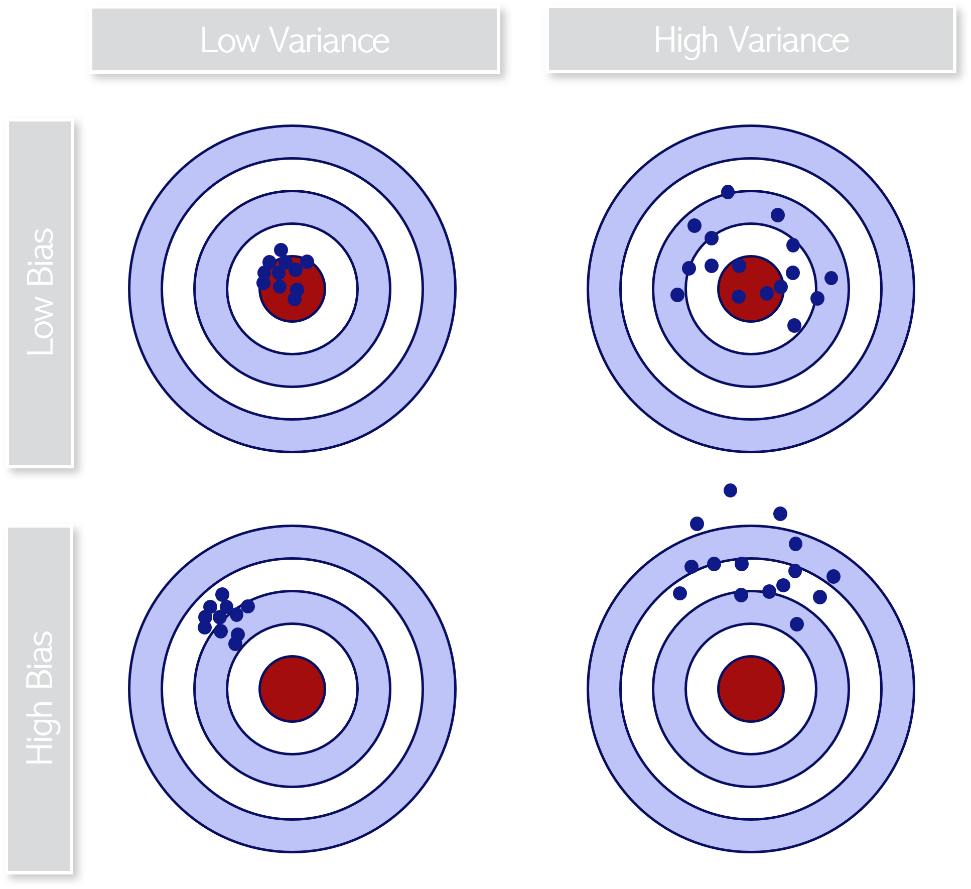
\(Variance_i = (y_i - \hat{y})^2\)
We usually aim at maintaining a low variance for our model since that implies proper fit regardless of the given training set.
Underfitting
Underfitting is a common problem that occurs when a machine learning model is not complex enough to capture the underlying patterns in the data.
This can result in the model performing poorly on both the training set and the test set, as it fails to capture the relationships between the input features and the target variable.
Underfitting occurs when the model is too simple or has too few parameters relative to the complexity of the problem. For example, a linear regression model might underfit a dataset that has a non-linear relationship between the input features and the target variable, as it is not able to capture the curvature of the relationship.
Underfitting can be avoided by using more data and also reducing the features by feature selection. Reasons for Underfitting might be (1) high bias and low variance, (2) size of the training dataset used is not enough, (3) model is not complex enough, (4) training data contains too much noise.
Accordingly, underfitting can be reduced by increasing model complexity, increasing the number of features, feature engineering, removing noise or increasing the training data.
Overfitting
A statistical model is said to be overfitted when the model does not make accurate predictions on testing data.
Overfitting is a common problem that occurs when a machine learning model is too complex and fits the training data too closely, capturing noise or random fluctuations in the data instead of general patterns that would be useful for making predictions on new data. As a result, the model may perform well on the training set but poorly on new, unseen data.
Overfitting occurs when a model is too complex relative to the amount of training data available. When a model gets trained with so much data, it starts learning from the noise and inaccurate data entries in our data set and is not able to project those characteristics onto the new data.
Overfitting can be caused by (1) low bias and high variance, (2) the model containing too many insiginificant parameters, (3) the training data being too homogenous. Accordingly, overfitting can be reduced by includung regularization terms to reduce model complexity, amending the training dataset or applying cross-validation techniques.
5.3.2 Loss functions
A loss function is a mathematical function that measures the difference between the predicted output and the actual output for a particular input in a machine learning model. The loss function provides a measure of how well the model is performing on the training data, the overall goal of training the model is to minimize the loss function.
A fast set of loss functions does exist and their specification is not absolut plus highly dependent on the learning problem. The following table provides a brief overview of the most common loss functions.
Mean-squared errorThis is a common loss function used in regression problems, which measures the average squared difference between the predicted and actual values. The MSE loss function penalizes the model for making large errors by squaring them and this property makes the MSE cost function less robust to outliers.
\(MSE = \frac{1}{n} \sum_n (x_i - \overline{x})^2\)
Mean-absolute error
Another common loss function used in regression problems, which measures the average absolute difference between the predicted and actual values.
We define MAE loss function as the average of absolute differences between the actual and the predicted value. It’s the second most commonly used regression loss function.
It measures the average magnitude of errors in a set of predictions, without considering their directions.
The MAE loss function is more robust to outliers compared to the MSE loss function.
Therefore, you should use it if the data is prone to many outliers.
\(MAE = \frac{1}{n} \sum_n |x_i - \overline{x}|\)