Chapter 3 Reading, analysing, and manipulating data
Here, we cover how to read in data, different ways of storing data, how to plot it, and how to manipulate it. First, we start with the basics - setting up a data frame (like an excel sheet or pandas dataframe) and a matrix. Second, we show how to select and use subsets of your the data based on conditions. Third, we present some basic ways to summarise your data - summary tables and plots. We finish by taking a quick look at some more advanced objects called data tables, and taking a quick look at the packages in the ‘tidyverse,’ which are designed to allow you to quickly ad easily split, apply, and recombine data.
For illustration, we use a real life dataset from (Dell and Querubin (2018) ‘Nation Building Through Foreign Intervention: Evidence from Discontinuities in Military Strategies’)[https://dell-research-harvard.github.io/projects/492bombing]. This paper measures the effect of increased US firepower on support for insurgents in South Vietnam during the Vietnam war. In this section, we simply manipulate the data. In the section on modeling, we look at some relationships in this data.
3.1 Reading in datasets as dataframes
The basic way to work with a dataset in R is to use an object called a dataframe. At its core, a dataframe is like a table where each column is a vector. It is the R equivalent to the pandas objects in Python. Intuitively, it looks a bit like a spreadsheet with column headers.
To read in a file as a given data type, first you need to read the file. Typically, data will
come in csv files. The command to read them is read.csv. There are equivalents
for xls and dta files.
# lets read in a new dataframe

# To download the original data, go to
# https://scholar.harvard.edu/files/dell/files/nationbuilding.pdf
# The file we will use is there as `firstclose_post.dta'

# read.csv allows us to read a csv file into R. The `as.data.frame' wrapper
# tells R that we want the object to be represented as a dataframe

df <- as.data.frame(read.csv("vietnam_war.csv", stringsAsFactors = F))
One thing that can be unintuitive is how this treats strings. By default, R assumes
that any strings in your dataset are factors,
so will turn them into a factor variable. This can cause a lot of weird problems
when trying to slice. So I recommend starting by setting StringsAsFactors==F, and
then manually changing strings back into factors if you need them.2
Once you have read the data, use as followed by the name of your data type to put
it in the data type you want. as.data.frame has a series of different arguments allowing you to set
the column names, the row names, and so on.
A lot of older economists still use Stata. In Stata, you have to store
the data files in a format called a .dta file. To read these into R, use the
read_dta command in the `haven’ package.
# we explain how to read in packages in the next section - if you need to
# read a .dta file you should go and look at that section first
# library(haven)
# df <- as.data.frame(read_dta("firstclose_post.dta"))
Stata can be as simple as R for small operations, but can get very messy very quickly if you have to do anything more complex. To see this in practice, go and have a look at how many files Dell and Querubin have to use to compute the estimates in their paper.
We can have a quick look at the top rows in our dataframe using head.
# looking at the top of the dataframe

# only selecting the first ten columns for ease of reading
# code to look at all of them would be head(df)

head(df[,c(1:10)])
## X usid fr_strikes_mean fr_forces_mean pop_g naval_attack
## 1 0 101010101 0.6000000 0.6666667 -0.7473872 0
## 2 1 101010102 0.3703704 0.5555556 -0.4082199 0
## 3 2 101010103 0.3703704 0.5555556 -0.3186806 0
## 4 3 101010104 0.3750000 0.5000000 -0.5415232 0
## 5 4 101010105 0.3703704 0.5555556 -0.4552453 0
## 6 5 101010201 0.7222222 1.0000000 -1.7762434 NA
## sh_pf_presence sh_rf_presence fr_init fw_init
## 1 0.00000000 0.00000000 0.00000000 0
## 2 0.96296300 0.00000000 0.03703704 0
## 3 0.03703704 0.07407408 0.03703704 0
## 4 0.12500000 0.00000000 0.00000000 0
## 5 0.66666670 0.00000000 0.03703704 0
## 6 0.50000000 0.00000000 0.00000000 0Find the column names using colnames.
# what are the columns called?
# Again only printing first ten for ease - code for all would be
# colnames(df)

colnames(df)[1:10]
## [1] "X" "usid" "fr_strikes_mean" "fr_forces_mean"
## [5] "pop_g" "naval_attack" "sh_pf_presence" "sh_rf_presence"
## [9] "fr_init" "fw_init"# lets read in a new dataframe
# read.csv allows us to read a csv file into R. The `as.data.frame' wrapper
# tells R that we want the object to be represented as a dataframe
# For illustration, we are going to use some of the data from Dell and Querubin (2017)
# `Nation building through foreign interventions'. This estimates the causal effect of
# military firepower on insurgent support on the intensive margin
# discontinuities in US strategies across regions in South Vietnam during their
# occupation. We have observations by hamlet
# To download the original data, go to
# https://scholar.harvard.edu/files/dell/files/nationbuilding.pdf
# The file we will use is there as `firstclose_post.dta'
df <- as.data.frame(read.csv("vietnam_war.csv", stringsAsFactors = F))
# a lot of older economists still use Stata. In Stata, you have to store
# the data files in a format called .dta file. To read these into R, use the
# read_dta command in the `haven' package
# library(haven)
# df <- as.data.frame9(read_dta("firstclose_post.dta"))
# looking at the top of the dataframe
# only selecting the first ten columns for ease of reading
# code to look at all of them would be head(df)
head(df[,c(1:10)])## X usid fr_strikes_mean fr_forces_mean pop_g naval_attack
## 1 0 101010101 0.6000000 0.6666667 -0.7473872 0
## 2 1 101010102 0.3703704 0.5555556 -0.4082199 0
## 3 2 101010103 0.3703704 0.5555556 -0.3186806 0
## 4 3 101010104 0.3750000 0.5000000 -0.5415232 0
## 5 4 101010105 0.3703704 0.5555556 -0.4552453 0
## 6 5 101010201 0.7222222 1.0000000 -1.7762434 NA
## sh_pf_presence sh_rf_presence fr_init fw_init
## 1 0.00000000 0.00000000 0.00000000 0
## 2 0.96296300 0.00000000 0.03703704 0
## 3 0.03703704 0.07407408 0.03703704 0
## 4 0.12500000 0.00000000 0.00000000 0
## 5 0.66666670 0.00000000 0.03703704 0
## 6 0.50000000 0.00000000 0.00000000 0# what are the columns called?
# Again only printing first ten for ease - code for all would be
# colnames(df)
colnames(df)[1:10]## [1] "X" "usid" "fr_strikes_mean" "fr_forces_mean"
## [5] "pop_g" "naval_attack" "sh_pf_presence" "sh_rf_presence"
## [9] "fr_init" "fw_init"# we will mainly use the variable fr_strikes_mean - the average number of
# months in the given quarter with at least one airstrike
# lets add a column to a dataframe - the square of foreign airstrikes
df[["fr_strikes_mean_squared"]] <- df[["fr_strikes_mean"]]**2
# say the new variable is a vector vec - then we have to create it as a vector
# first and then add it as so
#vec <- c(1:length(df[,1]))
#df[["new_variable"]] <- vec
# lets check it actually is there
vec <- df[["fr_strikes_mean"]]**2
# and see if we produced any
# we can bind on new columns or rows to the outside using cbind and rbind
df <- cbind(df, vec)
#df <- rbind(df, vec)
# we can rename a column by position using `names(name of dataframe)[number of column]'
names(df)[1] <- "X"
# lets create a dataframe from two variables using cbind
# creating two vectors of the same length
vec <- c(1:10)
vec2 <- c(11:20)
# now, if they are the same length, we can cbind them together,
# then use as.data.frame to turn them into a dataframe. We can pass arguments
# such as column names etc directly to this - see the documentation for
# data frames for more information
df_2 <- as.data.frame(cbind(vec, vec2), columns=c("var1", "var2"))3.2 Slicing dataframes
The most useful thing to know about dataframes is how to slice them. This is how we extract the data we want to use in regression models etc. Dataframes behave as we might expect, knowing that they are made up of linked vectors. The syntax for slicing is df[row, column]. We can slice by position, as for vectors above, or by passing vectors of column names (e.g column names). If we want to select all rows/columns, we leave the appropriate entry blank. To extract a single column as a vector, we use double square brackets containing the column name as a string.
# slicing

sl_1 <- df[,1]
sl_2 <- df[c(3:4), c(1,2)]
sl_3 <- df[,c("usid", "fr_forces_mean")]

# lets find a single column
sl_4 <- df[["yr"]]

# you might also see people do this with a dollar sign like so
#df$yr
# but apparently this is less robust to exceptions. If you are more interested
# in this, see the section on slicing in `Advanced R' by Hadley Wickham.
Including square brackets after the syntax above allows us to add additional conditions for slicing. This can be very powerful, as we can select columns and then use logical conditions to slice our dataframe based on the values of the columns.
# Looking only at the hamlets that are buddhist
df_budd <- df[df[["buddhist"]]==1,]

# Only the hamlets that had less than half of months with at least one airstrike
# in quarters in 1971

df_2 <- df[df[["fr_strikes_mean"]]<0.5 & df[["yr"]]==1971,]

# Now any hamlets that existed in 1971 or had less than half of months with one airstrike

df_3 <- df[df[["fr_strikes_mean"]]<0.5 | df[["yr"]]==1971,]

# lets extract the mean number of months with foreign force engagments in those hamlets using a square
# bracket after we select the vector. Note, we are only passing a logical in the
# final bracket, so we omit the comma that indicates the dimension
# above

forces <- df[["fr_forces_mean"]][df[["fr_strikes_mean"]]<0.5 & df[["yr"]]==1971]

# This returns the entries of the vector fr_forces_mean, where the corresponding
# logicals are fulfilled. Thus, we get a vector of entries. Now lets take the
# mean of this.
mean(forces)
## [1] 0.36982623.3 Basic summary statistics
Once we have our dataset, we should summarise it. This allows us to eyeball any trends, see any patterns or weird features that we might have missed, and so on. These are common in empirical applications.3 Here, we will show you how to create a summary table and convert it to tex code, plot a histogram, and a line chart.
The most basic way to summarise your data is to use the base `summary’ command. This is a generic way of summarising many different R objects. Passing a dataframe of numerical variables gives the quantiles and mean of each column, as well as the number of NAs. Passing factors gives a frequency table of the frequency of each factor.
library(stargazer)##
## Please cite as:## Hlavac, Marek (2018). stargazer: Well-Formatted Regression and Summary Statistics Tables.## R package version 5.2.2. https://CRAN.R-project.org/package=stargazer# Lets summarise the first twelve columns of our dataset
df_for_summary <- df[,c(1:12)]
sum_1 <- summary(df_for_summary)To do this in a more flexible way, we can apply summary functions to the
data using sapply'.sapply’ is a member of the `apply’ family of functions
that takes as an input a dataframe or matrix and iterates over the columns. It
returns a dataframe or matrix object depending which we passed it.
# computing the mean of each column, omitting any NA observations

sapply(df_for_summary, FUN=mean, na.rm=T)
## X usid fr_strikes_mean fr_forces_mean pop_g
## 6.103000e+03 2.999219e+08 2.623032e-01 4.394916e-01 -2.679248e-02
## naval_attack sh_pf_presence sh_rf_presence fr_init fw_init
## 3.376539e-03 3.217444e-01 7.901538e-02 3.582017e-01 1.535283e-02
## en_d fw_d
## 8.612760e+00 6.300729e-02sapply(df_for_summary, FUN=sd, na.rm=T)## X usid fr_strikes_mean fr_forces_mean pop_g
## 3.524002e+03 1.258183e+08 3.073952e-01 3.249269e-01 1.996891e-01
## naval_attack sh_pf_presence sh_rf_presence fr_init fw_init
## 2.358882e-02 3.231069e-01 1.785427e-01 3.131460e-01 5.263280e-02
## en_d fw_d
## 3.879940e+01 2.004662e-01Neither of these look very nice however. The package ‘stargazer’
allows us to create nice looking tables in R that we can save or export. It
can even output the table as a tex file, that we can use directly in our Latex
documents. This package contains the function stargazer, which is a general
function we can use to create nice-looking summary and regression tables. It has
a lot of arguments we can use to create tables in different formats, including
different things etc. We change what summary statistics we display by passing a
vector of their names as characters to the summary.stat argument.
stargazer(df_for_summary, type="html")| Statistic | N | Mean | St. Dev. | Min | Pctl(25) | Pctl(75) | Max |
| X | 12,207 | 6,103.000 | 3,524.002 | 0 | 3,051.5 | 9,154.5 | 12,206 |
| usid | 12,207 | 299,921,922.000 | 125,818,263.000 | 101,010,101 | 207,082,903.0 | 434,030,755.0 | 492,010,602 |
| fr_strikes_mean | 12,207 | 0.262 | 0.307 | 0.000 | 0.000 | 0.444 | 1.000 |
| fr_forces_mean | 12,207 | 0.439 | 0.325 | 0.000 | 0.167 | 0.708 | 1.000 |
| pop_g | 11,967 | -0.027 | 0.200 | -6.853 | -0.008 | 0.018 | 4.520 |
| naval_attack | 11,545 | 0.003 | 0.024 | 0.000 | 0.000 | 0.000 | 0.500 |
| sh_pf_presence | 12,146 | 0.322 | 0.323 | 0.000 | 0.000 | 0.625 | 1.000 |
| sh_rf_presence | 12,146 | 0.079 | 0.179 | 0.000 | 0.000 | 0.037 | 1.000 |
| fr_init | 12,200 | 0.358 | 0.313 | 0.000 | 0.091 | 0.600 | 1.000 |
| fw_init | 12,200 | 0.015 | 0.053 | 0.000 | 0.000 | 0.000 | 0.556 |
| en_d | 12,200 | 8.613 | 38.799 | 0.000 | 0.500 | 5.547 | 923.667 |
| fw_d | 12,200 | 0.063 | 0.200 | 0.000 | 0.000 | 0.037 | 7.000 |
# now lets just have a look at the mean and sd

stargazer(df_for_summary, type="html", summary.stat = c("mean", "sd"))| Statistic | Mean | St. Dev. |
| X | 6,103.000 | 3,524.002 |
| usid | 299,921,922.000 | 125,818,263.000 |
| fr_strikes_mean | 0.262 | 0.307 |
| fr_forces_mean | 0.439 | 0.325 |
| pop_g | -0.027 | 0.200 |
| naval_attack | 0.003 | 0.024 |
| sh_pf_presence | 0.322 | 0.323 |
| sh_rf_presence | 0.079 | 0.179 |
| fr_init | 0.358 | 0.313 |
| fw_init | 0.015 | 0.053 |
| en_d | 8.613 | 38.799 |
| fw_d | 0.063 | 0.200 |
# Lets flip the axes

stargazer(df_for_summary, type="html", summary.stat = c("mean", "sd"), flip = T)| Statistic | X | usid | fr_strikes_mean | fr_forces_mean | pop_g | naval_attack | sh_pf_presence | sh_rf_presence | fr_init | fw_init | en_d | fw_d |
| Mean | 6,103.000 | 299,921,922.000 | 0.262 | 0.439 | -0.027 | 0.003 | 0.322 | 0.079 | 0.358 | 0.015 | 8.613 | 0.063 |
| St. Dev. | 3,524.002 | 125,818,263.000 | 0.307 | 0.325 | 0.200 | 0.024 | 0.323 | 0.179 | 0.313 | 0.053 | 38.799 | 0.200 |
# Lets create some tex code to use in our tex files, and save it as a tex file

stargazer(df_for_summary,out = "summary_stats.tex",summary.stat = c("mean", "median", "sd"),
          title = "Partial summary statistics - Dell and Querubin (2018)", digits = 2,
float.env = "table", notes = "")We can create a histogram of numerical variables by using the base R hist command.
We have to make sure to specify a number of bins when we do this, using the breaks
argument.
# Lets look at the distribution of the number of mean monthly airstrikes across
# South Vietnamese hamlets in 1971
airstrikes <- df[["fr_strikes_mean"]][df[["yr"]]==1971]
hist(airstrikes, breaks=20, col="lightblue", main="Mean months with scheduled airstrikes on South Vietnamese hamlets, 1971")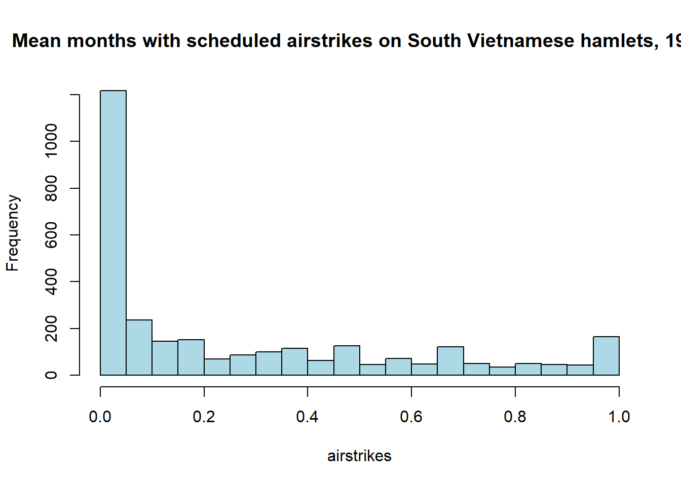 We can also plot any two variables against each other by using the base
 plot
command. The first argument is the variable on the x axis, the second argument
is the variable on the y axis. The type argument allows you to specify whether
you want a scatterplot, a line plot, or other types of plot. Additional arguments
allow us to specify the size of the points, the colour, axis sizes, titles, and
so on.
We can make more complex plots by creating a plot object, and then building on
top of it. I give an example of a more complex plot below. We start with a single
plot, containing a single line. We also specify some labels, a title, and control
the size of the text in general and axis labels in particular (using the cex arguments).
This is the first line of code in this base plot.
Next, we build it up a single element at a time, adding a new line of code below
for each element. We first plot two additional lines with line. We then manually
control each of the axes with axis. Passing the xact="n" and yact="n" commands
to the first plot allow us to do this.
# plotting the relationship between mean foreign forces and mean airstrikes in
# a hamlet over all years
plot(df[["fr_forces_mean"]], df[["fr_strikes_mean"]], type = "p", col="lightblue",
     pch = 19,
     xlab = "Mean months with foreign forces", ylab = "Mean months with airstrikes", main= "Mean months with foreign
     forces vs. mean months with scheduled airstrikes by quarter")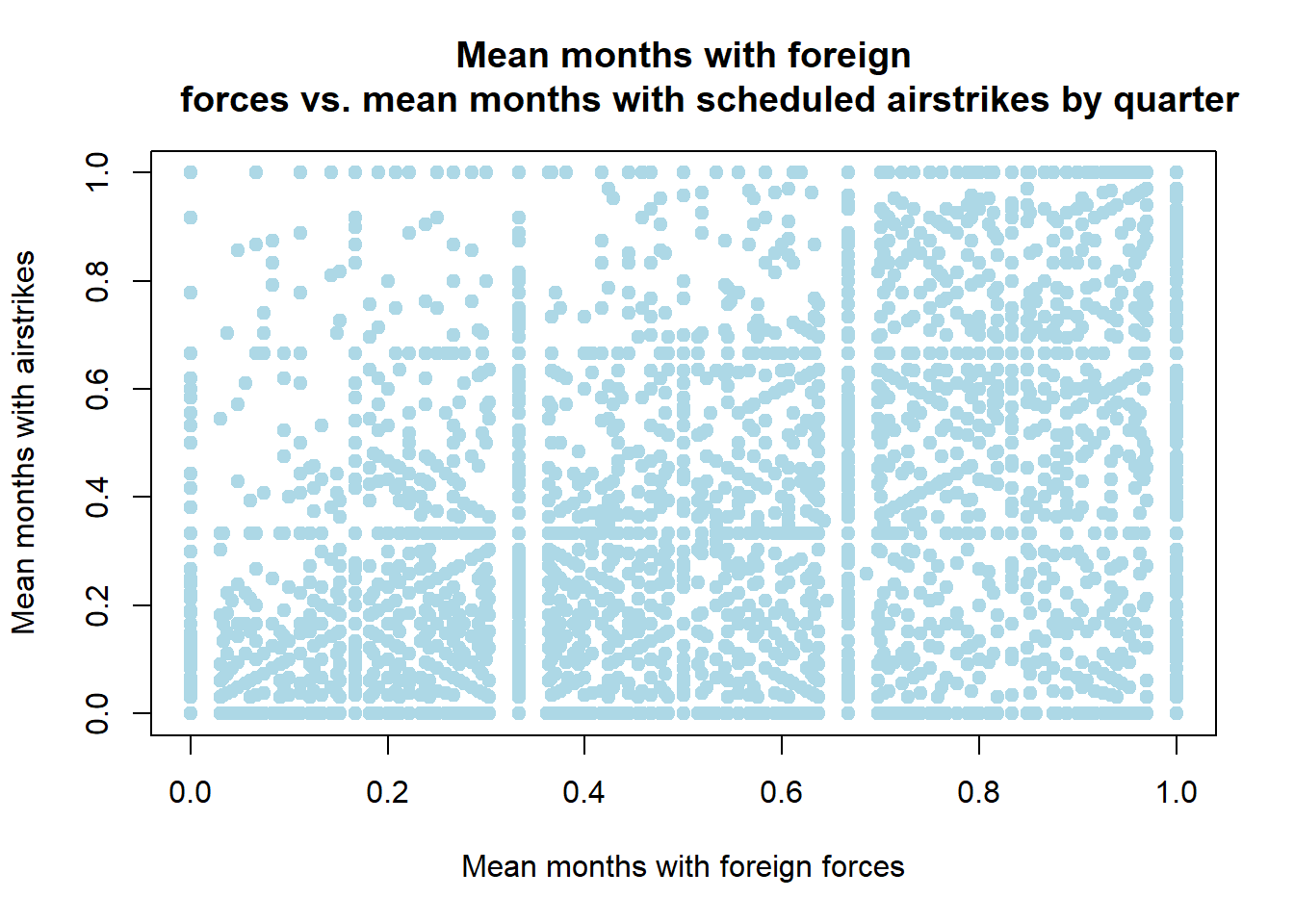
# now lets plot the mean airstrikes, ground operations, and naval strikes by year
# this will illustrate the basics of how to make more complex plots with base R
# Also this is a nice illustration how to use functions in lappply
# inputs: list of unique times in the dataframe,
# dataframe with at least two columns - time and thing we want to summarise,
# name of column representing units of time in the dataframe, and
# name of column we want to summarise
# outputs: list of means of column by year
mean_by_year <- function(time, df, name_of_year_column, name_of_summary_column){
obs_by_year <- df[[name_of_summary_column]][df[[name_of_year_column]]==time]
return(mean(obs_by_year, na.rm=T))
}
times_list <- as.list(unique(df[["yr"]]))
# lapply automatically assumes the list is the first argument to the function
# thus, we need to specify the other arguments as arguments to lapply
mean_airstrikes <- lapply(times_list, FUN=mean_by_year, df=df,
name_of_year_column="yr", name_of_summary_column = "fr_strikes_mean")
# this gives us a list - we need to flatten it into a vector to plot it
# unlist does this
mean_airstrikes <- unlist(mean_airstrikes)
mean_troops <- lapply(times_list, FUN=mean_by_year, df=df,
name_of_year_column="yr", name_of_summary_column = "fr_forces_mean")
mean_troops <- unlist(mean_troops)
# now plotting the airstrikes by year
# note a common trap here! when we unlist the times_list, it comes out both unordered
# and as a factor vector! So, if we try to plot it just like this, we get an error.
# Instead, we need to unlist it, turn it into numbers, and then order the vector.
times <- sort(unique(df[["yr"]]))
plot(times, mean_airstrikes, col="red", type="l", xlab="Year", ylab="Engagements",
main = "Mean monthly engagements in South Vietnamese hamlets by type",
cex = 1, cex.lab = 1.25, xaxt="n", yaxt="n", ylim = c(0.25, 0.5))
axis(2, at = seq(0, 1, by = 0.1), las = 1, cex.axis = 1.25)
axis(1, at = seq(1970, 1972, by = 1), cex.axis = 1.25)
lines(times, mean_troops, col="blue")
axis(2, at = seq(0, 1200, by = 100), las = 1, cex.axis = 1.25)
legend("topleft", legend = c("Mean airstrikes per month", "Mean troop engagements per month"),
pch=19, col = c("red", "blue"), cex = 1)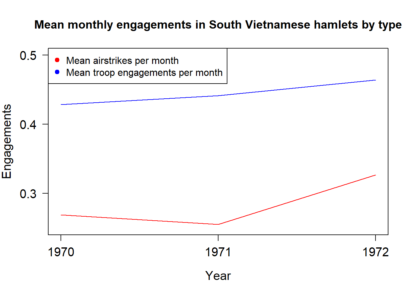 We can save any plot as a png file automatically by wrapping it in
png() and dev.off as above.
3.4 Summarising with the tidyverse - dplyr and ggplot2
The tidyverse system of libraries can make summarising and plotting data very easy - especially if it involves grouping the data. They also make complex operations more easily readable. It does this by adopting a different grammar to how standard R looks, and by being ‘opinionated’ - i.e making automatic decisions about a lot of defaults. The downside to this is that you have to be careful - the defaults can be different to what you would want - and you as the programmer have less control.
This is only a very very brief introduction to some tidyverse functions. If you like them, I would strongly recommend Hadley Wickham’s book ‘R for data science,’ which he has put in web form (here)[https://r4ds.had.co.nz/]. He is the creator of the tidyverse; and his books are really thorough, accessible, and well written.
3.4.1 Dplyr
There are six key dplyr functions: filter to select observations by values,
arrange to reorder rows, select to fetch columns by name, mutate to create
new columns from existing ones, group_by to fetch the values in one column that
depend on another, and summarise to compute summary statistics.
filter selects all the rows in a dataframe that satisfy one or more conditions.
The first argument is the dataframe; the subsequent arguments are logical conditions.
You do not need to put column names in quotes in this, and all, tidyverse functions.
It returns a dataframe with only rows that satisfy this condition.
arange orders a dataframe in descending order by the values in a set of columns, in the order
that we pass the column names. The first argument is the dataframe. The subsequent
arguments are the column names. It returns an ordered dataframe.
select subsets a dataframe by column names. It is another way of doing the
slicing we did in base R above. The first argument is the dataframe. The subsequent
arguments are the column names we want to select. It returns a dataframe containing
only those columns.
mutate creates new columns that are functions of existing columns. It is another
way of doing the slicing and tranformation we did above. The first argument is
the dataframe. The subsequent arguments are the columns we want to create. It
returns a dataframe that is the original dataframe plus the columns we wanted to
create.
summarise creates a table of summary statistics. This is similar to the summary
command in base R. group_by, however, allows us to create summaries that depend
on the values of certain columns e.g mean airstrikes by year. This allows us to
easily get at more complex features of our data.
When we use tidyverse packages, we can chain operations using a pipe %>%. In words,
this command says ‘and then.’ This can be very powerful, as it allows us to
do lots of complex operations to dataframes in single sets of commands as opposed
to creating lots of intermediate objects, or using messier nested functions.
# filter selects all the v
# first argument is the dataframe, second argument is the column value you want
# to filter by

library(tidyverse)
## -- Attaching packages --------------------------------------- tidyverse 1.3.0 --## v ggplot2 3.3.5 v purrr 0.3.4
## v tibble 3.0.4 v dplyr 1.0.2
## v tidyr 1.1.2 v stringr 1.4.0
## v readr 1.4.0 v forcats 0.5.0## Warning: package 'ggplot2' was built under R version 4.0.5## -- Conflicts ------------------------------------------ tidyverse_conflicts() --
## x dplyr::filter() masks stats::filter()
## x dplyr::lag() masks stats::lag()filtered_df <- filter(df, yr==1972)
arranged_df <- arrange(df, yr, usid)
selected_df <- select(df, usid, yr, fr_forces_mean)
mutated_df <- mutate(df, fr_strikes_mean_squared = fr_strikes_mean**2)
grouped_df <- group_by(df, yr)
summarise(grouped_df, count=n(), mean_forces = mean(fr_forces_mean))## `summarise()` ungrouping output (override with `.groups` argument)## # A tibble: 3 x 3
## yr count mean_forces
## <dbl> <int> <dbl>
## 1 1970 8571 0.441
## 2 1971 2989 0.429
## 3 1972 647 0.464# Combining both of these to do some powerful summarising
df %>% select(usid, yr, fr_forces_mean, fr_strikes_mean, naval_attack) %>%
group_by(as.factor(yr)) %>% summarise(count=n(), mean_forces = mean(fr_forces_mean),
mean_airstrikes = mean(fr_strikes_mean),
mean_naval_attack = mean(naval_attack)) ## `summarise()` ungrouping output (override with `.groups` argument)## # A tibble: 3 x 5
## `as.factor(yr)` count mean_forces mean_airstrikes mean_naval_attack
## <fct> <int> <dbl> <dbl> <dbl>
## 1 1970 8571 0.441 0.255 NA
## 2 1971 2989 0.429 0.269 NA
## 3 1972 647 0.464 0.327 NAggplot2 is the most common way to make plots in R. It is an easier
way to make beautiful plots than using the base plot and hist functions.
ggplot2 uses its own syntax, called the ‘grammar of graphics.’
In short, you create a base plot object, and then add additional things to it
using + signs afterwards.
In any ggplot, we start by passing ggplot(). This sets up the coordinate
system for what we want to summarise.
Next, we pass how we want to summarise it.
This can be in a lineplot, scatterplot, heatplot and so on. Each have their own
ggplot2 commands. Within that, or the ggplot() command, we have to specify a
mapping from the values in our dataset to the things on the plot.
We do this
with the mapping argument. We always pair this with an aes wrapper, within
which we specify the aesthetics for this plot - what is on the x axis, what is
on the y axis, and some other possible arguments. We can use these to colour the
points by characteristics, put them into different shapes, and so on as long as
these things map from the values of the points. There are other arguments, such
as general size colour, that are properties of the points but not of their values.
These go outside of the mapping argument.
This is the base ggplot uses to build the plots. Next, we can add arguments and layer up commands to build the type of the plot we want to make. There are many different ways that we can do this to make some incredibly clean and beautiful plots. For examples, see http://r-statistics.co/Top50-Ggplot2-Visualizations-MasterList-R-Code.html#Histogram.
# Lets start with the simplest thing - a scatter plot

ggplot(data = df[df[["yr"]]==1972,]) + geom_point(mapping = aes(x =fr_strikes_mean, y=en_prop))
## Warning: Removed 21 rows containing missing values (geom_point).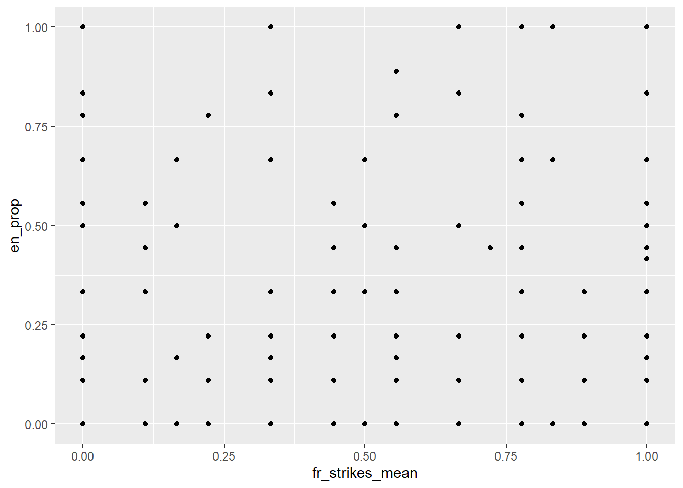
# lets change the colour of all of the points

ggplot(data = df[df[["yr"]]==1972,]) + geom_point(mapping = aes(x =fr_strikes_mean, y=en_prop), colour="orange")
## Warning: Removed 21 rows containing missing values (geom_point).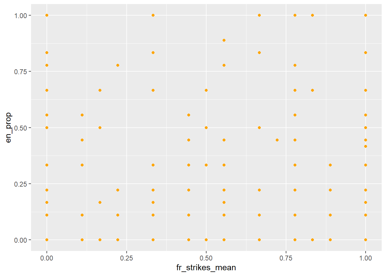
# now lets colour some points

ggplot(data = df[df[["yr"]]==1972,]) + geom_point(mapping = aes(x =fr_strikes_mean, y=en_prop, color = fr_forces_mean))
## Warning: Removed 21 rows containing missing values (geom_point).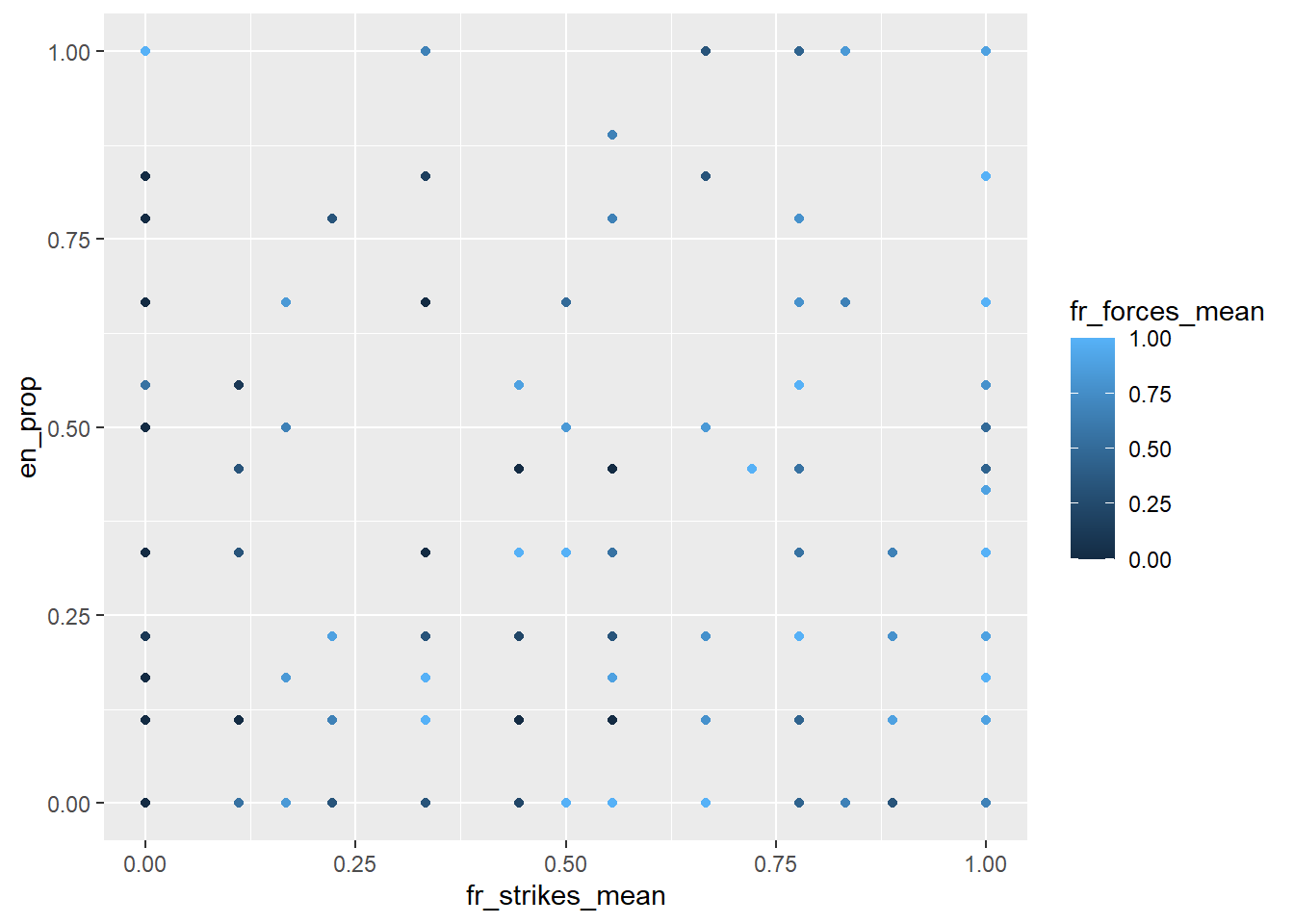
# we could also do this with, for example, size

ggplot(data = df[df[["yr"]]==1972,]) + geom_point(mapping = aes(x =fr_strikes_mean, y=en_prop, size = fr_forces_mean))
## Warning: Removed 21 rows containing missing values (geom_point).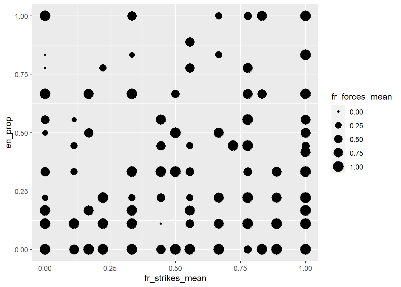
# now lets build up by adding a smoothed line through all of the points

ggplot(data = df[df[["yr"]]==1972,], mapping = aes(x =fr_strikes_mean, y=en_prop)) +
  geom_point() +
  geom_smooth()
## `geom_smooth()` using method = 'loess' and formula 'y ~ x'## Warning: Removed 21 rows containing non-finite values (stat_smooth).
## Warning: Removed 21 rows containing missing values (geom_point).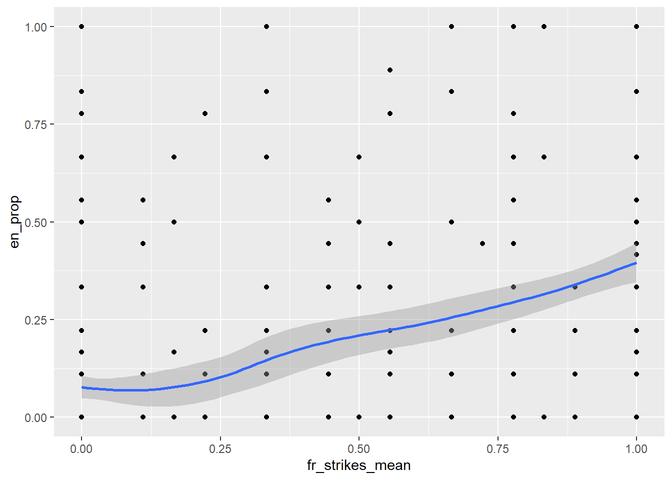
If you ever wonder why the default is
T, see https://simplystatistics.org/2015/07/24/stringsasfactors-an-unauthorized-biography/↩︎In the worst case, it can help uncover fraud - e.g https://datacolada.org/98.↩︎