Chapter 6 Advanced programming techniques
By this point, we have covered the basics of programming in R. Now we have done this, we will present a little more advanced material that can be useful and make your code better. These are based around programming your own estimators. First, we will show you how to simulate some data to use with Monte-Carlo simulation. We will use the vectorising tricks we learnt in the first section. Then, we will use this data to demonstrate optimisation in R. We will do this by programming a maximum-likelihood estimator. Finally, we will demonstrate how to speed up code by profiling it.
6.1 Advanced iteration and Monte-Carlo simulation
First, we will generate some of our own data to use by doing some Monte-Carlo simulations. This is a useful thing to be able to do by itself. Furthermore, we will use it to reinforce some of the principles of R we learned earlier, and introduce some more cool advanced features you might want to use. Here, we do not simulate our data in the most efficient way that we could. For some more advanced ways of doing so, see this great article by Grant McDermott.
We are generating some random numbers. So we should start by setting a seed for our
random number generator. Seeding sets the starting value for the random number
generators in your program. As random number generators are deterministic, setting
a seed ensures that you get the same random numbers each time that you run your code.
This helps with debugging, and ensures others can reproduce our code.
We can do this in R with set.seed().
# lets set a seed for reproducibility

rm(list=ls())

set.seed(854)
Next, we need to generate some random numbers. Base R has a lot of nice inbuilt commands for sampling from different distributions. The synatx is generally as follows. In the first argument, you specify the number of draws you want to make. In the next arguments, you specify the parameters of the distribution - e.g the mean and standard deviation for a normal distribution. R then outputs a numeric vector composed of draws from the distribution.
# Some examples of drawing random numbers in R

# the command 'runif' gives draws from a uniform [0,1] distribution if you do
# not specify a support

unif_1 <- runif(35)

# but you can specify a support, using the 'min' and 'max' parameters

unif_2 <- runif(35, min= 20, max= 40)

# the command 'rnorm' gives draws from a normal distribution with parameters 'mean', 'sd'

# lets do 20 draws from a standard normal distribution

norm_1 <- rnorm(20, mean=0, sd=1)

# the command rchisq gives draws from a chi-square distribution with degrees of
# freedom 'df'

chi_sq_1 <- rchisq(34, df=100)

# finally, rpois gives draws from a poisson distribution with rate parameter
# 'lambda'

pois_1 <- rpois(22, 6)
In general, the syntax for random number draws in R is composed of a root name, that we precede with a prefix from (p,q,d,r). The root name is a shorthand for the name of the distribution. P gives us the cumulative probability for a given value from the c.d.f, q gives us the inverse of the c.d.f (i.e quantiles), d gives us the probability mass from the density function, and r draws random numbers from the set distribution. For a list of the roots for common variables in R, see here.
Now we can generate some random numbers, we need to efficiently generate lots of them. For illustration, lets simulate a linear regression model in three variables. Each of the variables is itself normally distributed, and we have a normally distributed error term. We will also only do small simulations of 1000 data points for ease.
Our first instinct when doing something like this might be to just use a for or
while loop. We might also think that to store our values, we should initialise
an empty vector and then fill it with values.
# How not to do simulation in R

vec_x1 <- c()
vec_x2 <- c()
vec_x3 <- c()

i <- 0
while (i <100){

  vec_x1 <- c(vec_x1, rnorm(1, 2, 1))
  i <- i + 1
}

j <- 0
while (j <100){

  vec_x2 <- c(vec_x2, rnorm(1, 2, 1))
  j <- j + 1
}

k <- 0
while (k <100){

  vec_x3 <- c(vec_x3, rnorm(1, 2, 1))
  k <- k + 1
}
This is not a good way to go about this for two reasons.
Firstly, we do not want to do our simulation using loops because R is a vectorised language. Practically, being vectorised means that operations involving vectors are much much faster than loops. R is different in this way to other languages like Python and C++, which are object-oriented instead. In object-oriented languages, loops are very efficient and can even sometimes be faster than operations on vectors. As the amount of data we want to simulate here is small, this does not matter so much. It will begin to matter more if we try to simulate a lot more data, however.
Secondly, we do not want to store more data by expanding a vector. The way R
stores objects in memory makes this very memory intensive and inefficient. It is
much better to create an object of right length, and then replace the values
we need to use. We can create a vector of a given length using the rep function.
The first argument of this is some value. A good choice to use is NA, so we can
work out if our filling steps later fail. The second argument is the length of
the vector you want to produce.
Lets do the second first. We now reproduce one of the simulations above, but instead of growing a vector we create a vector of NAs, and then fill it up.
# Some more efficient, vectorised, simulation code

# creating empty vectors with rep

vec_x1 <- rep(NA, 100)

i <- 0
while (i <100){

  # note we have to use i+1 here as we start at 0, but R starts counting lengths
  # at 1
  vec_x1[i+1] <- rnorm(1, 2, 1)
  i <- i + 1
}
Next, lets replace the loop. We already know that we can draw vectors of random variables directly. We might not be able to do this if our use case is a bit more complicated though. Thus, we should also look at applying a function to generate the data. We will do this by generating 100 sets of our observations, storing these as a dataframe, and then applying a function to fit regression models to these observations.
#--------------------------------------------------------------------------------
# Some more efficient Monte-Carlo
# Say we want to find the distribution of the estimates of \beta_{1} in a
# linear regression model of the form y_{i}= \alpha + \sum_{j}\beta_{j}x_{i}^{j} + e_{i}
# up to the third order
#--------------------------------------------------------------------------------
# Parameters -------------------------------------------------------------------
# Number of simulations
mc <- 100
# Number o data points within each simulation
length_within_sim <- 100
# 'True parameters' of the regression model
alpha = 2.2
beta_1 = 0.5
beta_2 = 0.3
beta_3 = 0.2
# Functions -------------------------------------------------------------------
# here we are going to group our dataframe by a group indicator, and
# then fit the linear regression to subsets of the data by the group
# indicator
fit_reg <- function(group, group_col, df, reg_formula){
# note that it is acutally more efficient here to use the lm.fit
# method - if you would like to do something more advanced take
# a look at that with ?lm.fit
mod <- lm(reg_formula, data=mc_df[mc_df[[group_col]]==group,])
return(mod[["coefficients"]][2])
}
# Running code -----------------------------------------------------------------
# Generating our variables
int <- rep(mc*length_within_sim, alpha)
vec_x1 <- rnorm(mc*length_within_sim , 2, 1)
vec_err <- rnorm(mc*length_within_sim, 0,1)
# Here we are fitting a cubic function. Thus, we simulate the new
# variables by operating on the old ones. This is more efficient
# (Thanks to Katya Ugulava for pointing this out to me)
vec_x2 <- vec_x1^2
vec_x3 <- vec_x1^3
# now creating a group indicator for each of our simulations using the each
# command in rep
group <- rep(c(1:100),each=100)
# putting these ina dataframe to then fit the regression
mc_df <- as.data.frame(cbind(group, int, vec_x1, vec_x2, vec_x3))
names(mc_df) <- c("group","int", "x1", "x2", "x3")
# lets just change the rownames now for ease of use
# notice we are using fast vectorised multiplication here!
mc_df[["y"]] <- mc_df[["int"]] + beta_1 * mc_df[["x1"]] + beta_2 * mc_df[["x2"]] + beta_3 * mc_df[["x3"]] + vec_err
# finally, lets apply our fitting function above to the dataframe
# to get a set of estimates of \beta_{1}
beta_vec<- unlist(lapply(1:100, FUN=fit_reg, group_col="group", df=mc_df,
reg_formula = "y~x1+x2+x3"))
hist(beta_vec, breaks=25, col="red", main="Distribution of the estimator for beta_{1}")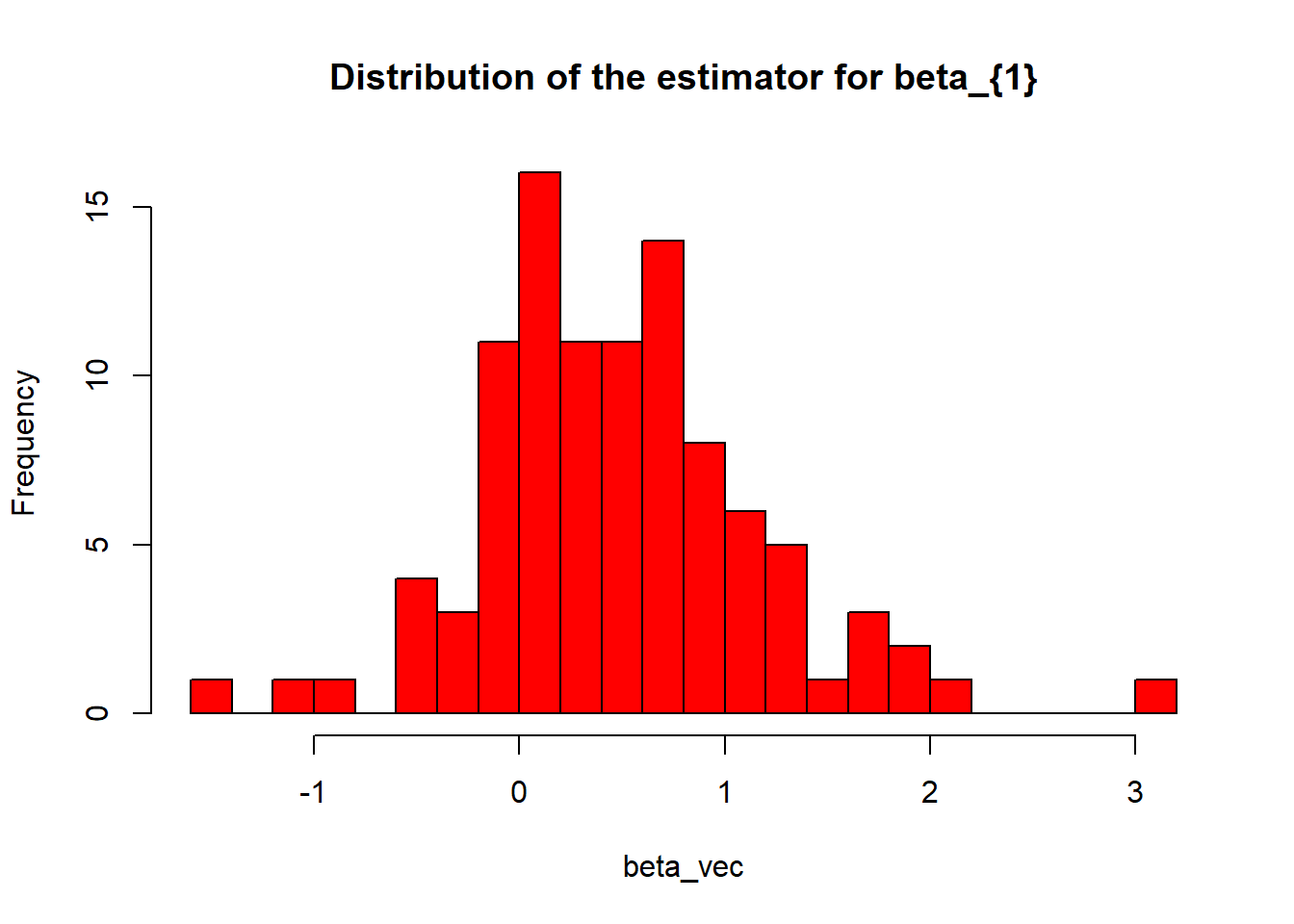 If we want to do this more times, we should write the whole Monte-Carlo operation
as a function where we pass the parameter values as an argument.
If we want to do this more times, we should write the whole Monte-Carlo operation
as a function where we pass the parameter values as an argument.
We can still make this more efficient though, by replacing our dataframe with
an object called a data.table or a tibble, and then doing something called
‘nesting’ the operation within the table. Here we cover how to do this with a
data.table - for tibbles see https://r4ds.had.co.nz/many-models.html .
A data.table is effectively an improved version of the base R data.frame. It
comes in its own package with the same name. data.tables keep the same functionality
as data,frames, but add the ability to perform operations on the rows and columns
as part of the object. We will demonstrate these functionalities while performing
our simulations. The most important of these is the by argument. by is an inbuilt
argument to group data by the values in a column within the data.table.
# Demonstrating some data table functionalities
# before performing our Monte-Carlo

library(data.table)

# lets generate some data and use it
# one random variable and two different
# groups

col_1 <- rnorm(10000, 0,1)
col_2 <- rep(c("A", "B"), each=5000)

# the command as.data.table allows us to convert an object into a data.table
# if we already have a dataframe or list object, we can use DT() instead

dt <- as.data.table(cbind(col_1, col_2))
names(dt) <- c("r_v", "grp")
# this code ensures our r_v column is a numeric variable
dt[,r_v :=as.numeric(r_v)]

# In addition to selecting columns by passing strings, in data.table we can now
# just select columns based on names
# data.table also recognises automatically which of our conditions are rows and
# column names, so we do not have to include the data.table name to carry out
# operations as in a data.frame

dt[r_v < -1 & grp =="A"]
## r_v grp
## 1: -1.703836 A
## 2: -1.674758 A
## 3: -1.641446 A
## 4: -1.029205 A
## 5: -1.831224 A
## ---
## 766: -1.729828 A
## 767: -1.713903 A
## 768: -1.821262 A
## 769: -1.930295 A
## 770: -1.403510 A# One inbuilt functionality is ordering!
# ordering lexically by group, and then by the value of the random variable
dt <- dt[order(r_v)]
# Some useful inbuilt functions
# .N counts the number of observations with a preceeding condition
dt[r_v<-1 & grp=="A", .N ]## [1] 5000# by allows us to start doing some aggregation
# lets compute the number of observations in each group
dt[,.N, by=grp]## grp N
## 1: A 5000
## 2: B 5000# we have to enclose custom functions in a bracket, and precede them with
# a . to apply them to all observations that satisfy any condition in
# the preceding argument
dt[,.(mean(r_v)), by=grp]## grp V1
## 1: A 0.009828461
## 2: B -0.012719875dt[r_v < -1,.(mean(r_v)), by=grp]## grp V1
## 1: A -1.521316
## 2: B -1.551410# we can chain these operations on the rows by adding [] containing a new
# operation after the end of our code above
dt[r_v < -1,.(mean(r_v)), by=grp][order(grp)]## grp V1
## 1: A -1.521316
## 2: B -1.551410Above, we only provide a brief overview of what data.tables can do. Also read
https://cran.r-project.org/web/packages/data.table/vignettes/datatable-intro.html .
Now lets use data.table to nest our Monte-Carlo routine. The idea of nesting is the
following. Typically, when we create an object like a data.frame or data.table,
we think of each entry as being a single thing like a number or word. But this does
not have to be the case. We can actually fill the entries in these objects with
other objects, like lists or data.tables. data.table provides us with a set
of inbuilt iteration operations that are more efficient than just using the
base apply over subsets of a given data.frame or data.table. Thus, by storing
subsets of our data as observations in our data.table we can exploit the inbuilt
iteration operations to do any iteration we want in a more efficient way.
If that sounds abstract, lets take a look at a concrete example by making our
Monte-Carlo code a bit more efficient. We will use the .SD inbuilt function
in data.table to create a data.table containing just nested subsets of our data
by the value of a variable (in our case, our group variable we make during the
simulation).
#--------------------------------------------------------------------------------
# Some even more efficient Monte-Carlo using nested operations in data.table
# Say we want to find the distribution of the estimates of \beta_{1} in a
# linear regression model of the form y_{i}= \alpha + \sum_{j}\beta_{j}x_{i}^{j} + e_{i}
# up to the third order
#--------------------------------------------------------------------------------


# Parameters -------------------------------------------------------------------

# Number of simulations
mc <- 100

# Number o data points within each simulation
length_within_sim <- 100

# 'True parameters' of the regression model

alpha = 2.2
beta_1 = 0.5
beta_2 = 0.3
beta_3 = 0.2

# Functions -------------------------------------------------------------------

# here we are going to group our dataframe by a group indicator, and
# then fit the linear regression to subsets of the data by the group
# indicator
fit_reg <- function(group, group_col, df, reg_formula){

  # note that it is acutally more efficient here to use the lm.fit
  # method - if you would like to do something more advanced take
  # a look at that with ?lm.fit
  mod <- lm(reg_formula, data=mc_df[mc_df[[group_col]]==group,])
  return(mod[["coefficients"]][2])

}

# Running the code -------------------------------------------------------------

# Generating our variables
int <- rep(mc*length_within_sim, alpha)
vec_x1 <- rnorm(mc*length_within_sim , 2, 1)
vec_err <- rnorm(mc*length_within_sim, 0,1)

# Here we are fitting a cubic function. Thus, we simulate the new
# variables by operating on the old ones. This is more efficient
# (Thanks to Katya Ugulava for pointing this out to me)

vec_x2 <- vec_x1^2
vec_x3 <- vec_x1^3

# now creating a group indicator for each of our simulations using the each
# command in rep

group <- rep(c(1:100),each=100)

# putting these in a dataframe to then fit the regression

mc_df <- as.data.table(cbind(group, int, vec_x1, vec_x2, vec_x3))
names(mc_df) <- c("group","int", "x1", "x2", "x3")

# lets just change the rownames now for ease of use
# notice we are using fast vectorised multiplication here!
mc_df[["y"]] <- mc_df[["int"]] + beta_1 * mc_df[["x1"]] + beta_2 * mc_df[["x2"]] + beta_3 * mc_df[["x3"]] + vec_err

# now lets define a data.table containing a new column 'data' which is our
# data subsetted by the value of the group variable
mc_dat = mc_df[, list(data=list(.SD)), by=group]

# now we can use the inbuilt data.table iterators to fit all of our regression
# models
# what this does here is define a new column (:=) by applyng the function
# from our function above to all of the elements x of the column
# As we do it within the data.table, it is really fast!
mc_dat[, model := lapply(data, function(x) lm(y ~ x1 + x2 + x3, x)[["coefficients"]][2])]

# now mc_dat[, model[[1]], by=group] gives us our data back as a column
# (automatic name V1) with the group. To plot it, we need to extract it as
# a vector. Thus, we slice it out just using standard dataframe syntax for ease.

hist(mc_dat[,model[[1]], by=group][["V1"]], breaks=25, col="red", main="Distribution of the estimator for beta_{1}")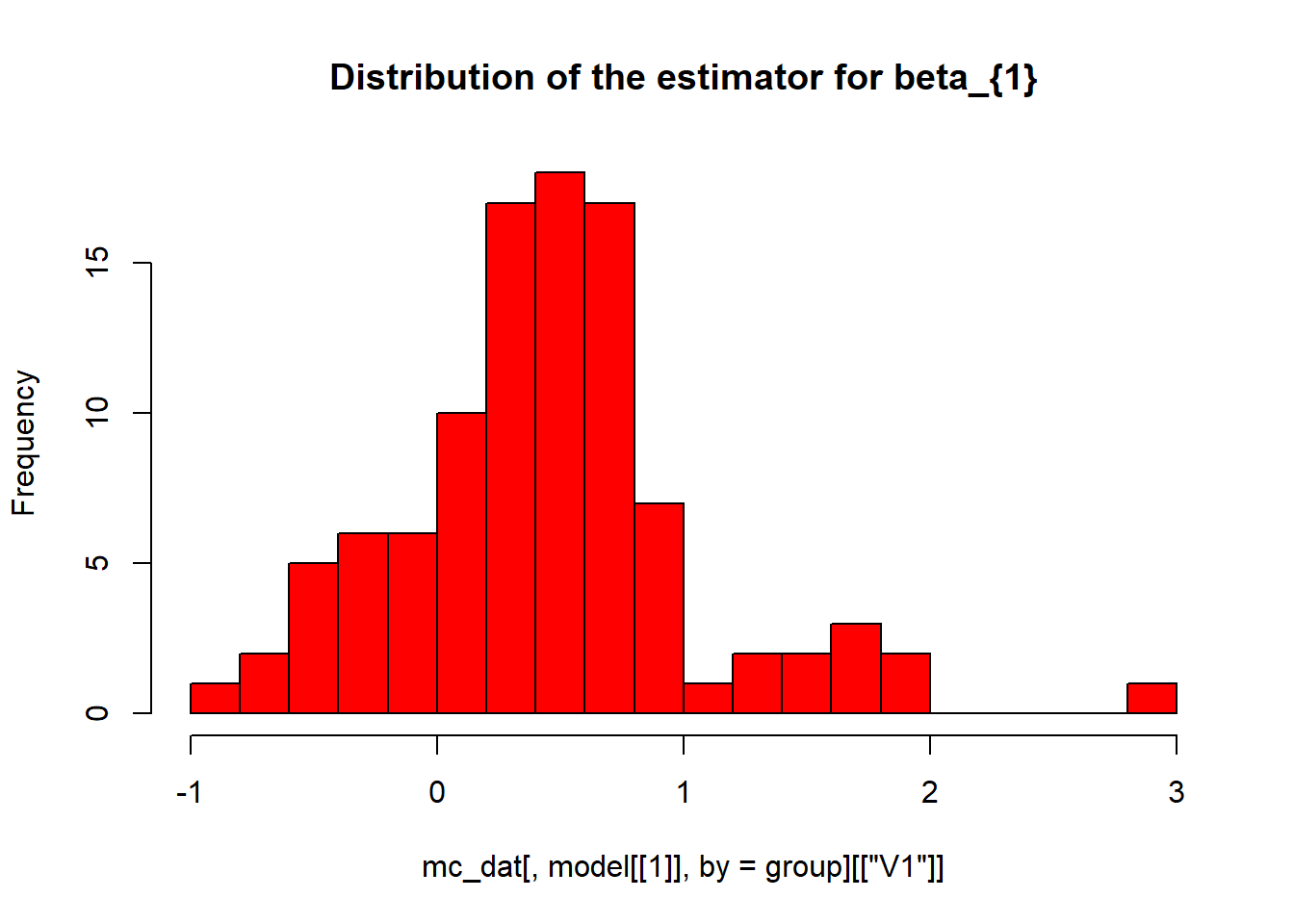
6.2 Optimisation
If we choose to program our own estimators, we often compute the value of the
estimator by maximising or minimising an objective function. Thus, we need to
know how to do optimisation in R. Here, we cover the basic way to do optimisation
in R using the optim function. As an example, we show how to program a maximum-likelihood
estimator from scratch (as opposed to using say mle).
The optim function in base R is a minimiser. It takes the value of a objective
function, which we write as a function. It then minimises the function using an
algorithm that we specify, given a starting value that we also specify. The first
argument is the starting value. The second argument is the function that we want
to minimise. The third argument is the method that we want to use to compute it.
The default method is the Nelder-Mead algorithm; value “BFGS” gives the BFGS
quasi Newton-Raphson algorithm. Adding hessian=T gives us the Hessian matrix
as an output.
When we write the function, the vector that we are trying to optimise must be the first argument of the function. We must return the value of the objective function that we are trying to minimise. Thus, if we want to maximise something, we must return the negative of that thing.
Lets try it out by programming the maximum likelihood estimator for a linear regression with normally distributed errors using the data from one of the runs of our Monte-Carlo simulation earlier.
# Example of optimisation in R - programming the maximum likelihood estimator
# for a linear regression with normally distributed errors
# Here I borrow from this guide https://www.ime.unicamp.br/~cnaber/optim_1.pdf

# we will minimise the negative log-likelihood (equivalent of course to
# maximising the normal likelihood function as the location of optima are
# preserved under monotonic transformations)

# we just do it for one parameter for ease

negative_log_likelihood <- function(param_vec, X_mat, y_vec){
  beta_vec <- param_vec[1:4]
  sigma2 <- param_vec[5]
  n <- nrow(y_vec)
  mu <-
  inner_sum <- sum((y_vec-X_mat %*% beta_vec)**2)
  log_l <- -0.5*n*log(2*pi) -0.5*n*log(sigma2) - (1/(2*sigma2))*sum((y_vec-X_mat %*% beta_vec)**2)
  return(-log_l)
}

beta_vec <- optim(c(0,0, 0, 0,1), negative_log_likelihood, method="BFGS", hessian = T,
                  X_mat = as.matrix(mc_df[mc_df[["group"]]==1,c(2:5)]),
                  y_vec = as.matrix(mc_df[mc_df[["group"]]==1,c(6)]))
## Warning in log(sigma2): NaNs producedbeta_vec## $par
## [1] 0.9999929 0.9724584 -0.2416691 0.3128821 3.5391276
##
## $value
## [1] 169.0368
##
## $counts
## function gradient
## 60 11
##
## $convergence
## [1] 0
##
## $message
## NULL
##
## $hessian
## [,1] [,2] [,3] [,4] [,5]
## [1,] 2.825555e+09 5.362870e+05 1.293351e+06 3.533071e+06 2.0816105462
## [2,] 5.362870e+05 1.293351e+02 3.533071e+02 1.054175e+03 0.0006779075
## [3,] 1.293351e+06 3.533071e+02 1.054175e+03 3.345331e+03 0.0022651463
## [4,] 3.533071e+06 1.054175e+03 3.345331e+03 1.111938e+04 0.0076538527
## [5,] 2.081611e+00 6.779075e-04 2.265146e-03 7.653853e-03 -1.7645778030We see here that this outputs the parameters, the value of the log-likelihood at the minimum, and then some additional statistics. As we selected the Hessian, we can compute the standard errors.
# We get the standard errors by taking the square root of the principal diagonal
# of the inverse of the Hessian

sqrt(diag(solve(beta_vec[["hessian"]])))
## Warning in sqrt(diag(solve(beta_vec[["hessian"]]))): NaNs produced## [1] 6.556477e-05 1.126158e+00 6.547648e-01 1.124175e-01 NaN6.3 Profiling
Imagine we want to make our code more efficient so it runs quicker. This may sound unnecessary, but it can be important in applied econometric. If we are working with large datasets with hundreds of thousands of rows and doing lots of iteration small inefficiencies can make our code run very slowly as we might be hitting them thousands and thousands of times.
The standard way to do this is by ‘profiling’ our code. The aim is to find the
biggest bottleneck we have not dealt with yet, deal with it as best we can, and
repeat until our code performs well enough. This might sound trivial. It is not.
Thus, programmers typically find the bottlenecks by iteratively testing and
timing sections of the code using small, manageable inputs. Here, we take a
short look at how to do this in R with the profvis package. For more details,
look at the chapter on this in Hadley Wickham’s ‘Advanced R’ (we follow the first
section of this chapter here).
# loading the library containing our profiler
library(profvis)
## Warning: package 'profvis' was built under R version 4.0.5f_1 <- function() {
pause(0.5)
f_2
}
f_2 <- function(){
print("hello world")
}
# we can profile by taking our function, and wrapping it in the function 'lineprof()'
# we wrap all of the code we want to profile in curly brackets {}
profvis({f_1()
f_2()})## [1] "hello world"The profvis function will open up an interactive profiler where we can
look at the relative speed of different parts of our code. This allows us to
isolate which bits of the code take more or less time. We can test different
versions by wrapping them in the profvis wrapper, and seeing if they take more
or less time.
# now make the pause slower
# we should see that it runs a lot quicker
f_3 <- function() {
  pause(0.25)
  f_2
}

# it does!

profvis({f_3()
  f_2()})
## [1] "hello world"