7 Statistical Fundamentals
library(readr)
library(tidyverse)
7.1 Intro
This tutorial details fundamental statistical concepts, illustrated with IBIS data. The main purpose is two-fold 1) to develop a set of notation, definitions, and ideas that comprise the foundamentals behind standard statistical analyses and 2) to introduce some basic statistical methods and illustrate how they are carried out in R using IBIS data. The notation and concepts developed here will be referenced again in later tutorials, so those without formal statistical training would be inclined to read this tutorial. For those with a solid background in statistics, this tutorial should serve as a quick refresher as well as an reference for standard statistical terminology and notation.
7.2 Statistical Inference
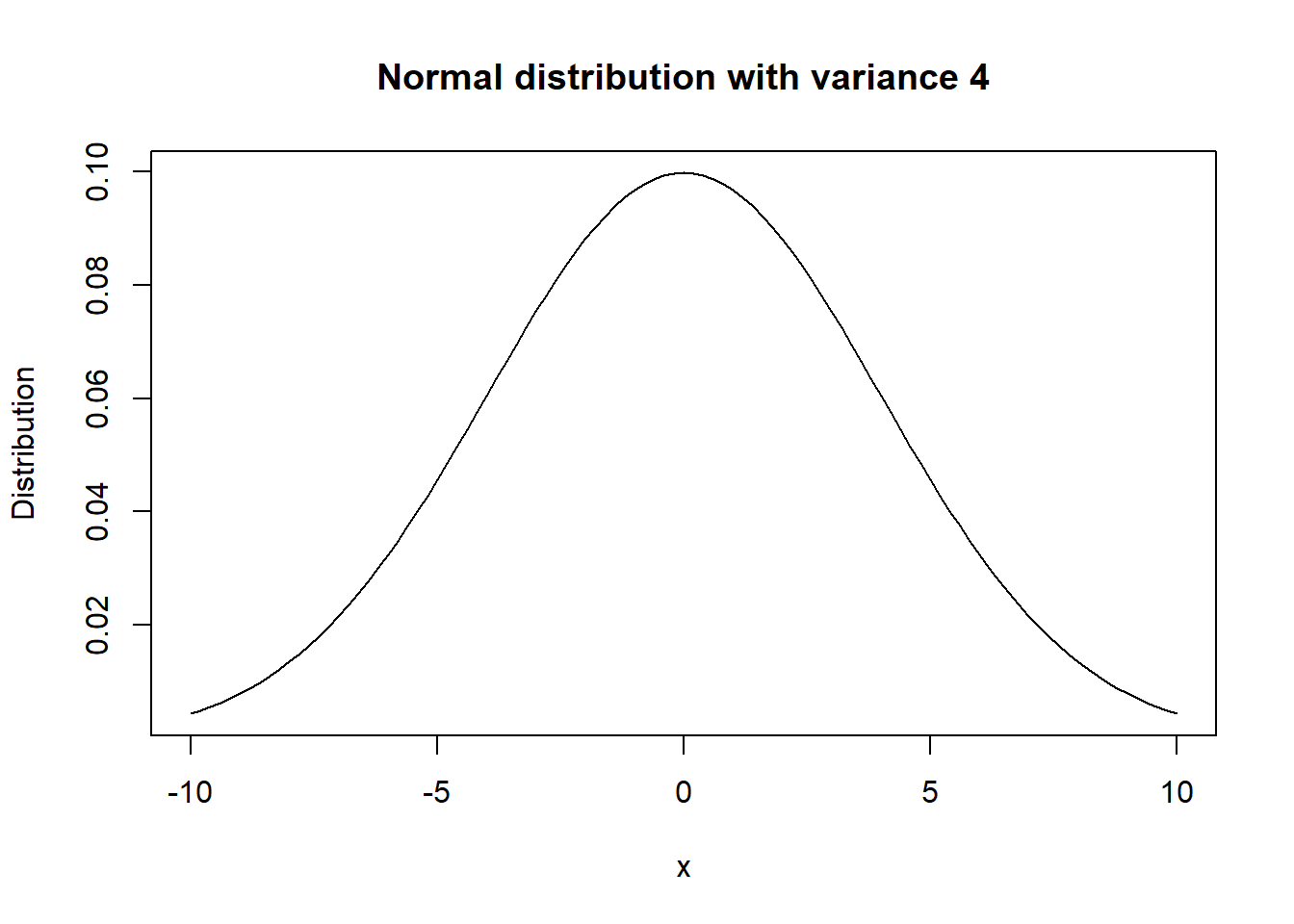
For variable \(X\), its distribution can be thought of as a function which states the probability of \(X\) equalling a specific value \(x\), for every possible \(x\). For example, if \(X\) is normal distributed, its distribution can be plotted as shown below.
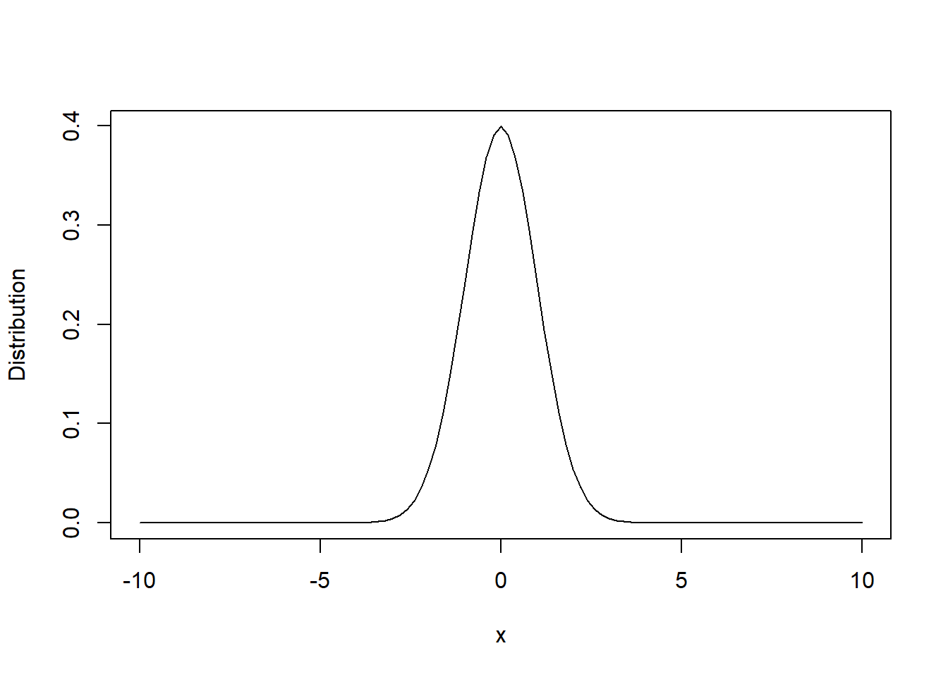
We can see that the probability is highest around \(x=0\), and then quickly decreases as you move away from \(0\). When given real data, often a histogram is used to visualize the variable’s distribution. For example, the histogram of AOSI total score 12 months in the AOSI cross sectional data is the following:
data <- read.csv("Data/Cross-sec_full.csv", stringsAsFactors=FALSE, na.strings = c(".", "", " "))
hist(data$V12.aosi.total_score_1_18, xlab = "AOSI Total Score",
     main="Histogram of AOSI Total Score at 12 months")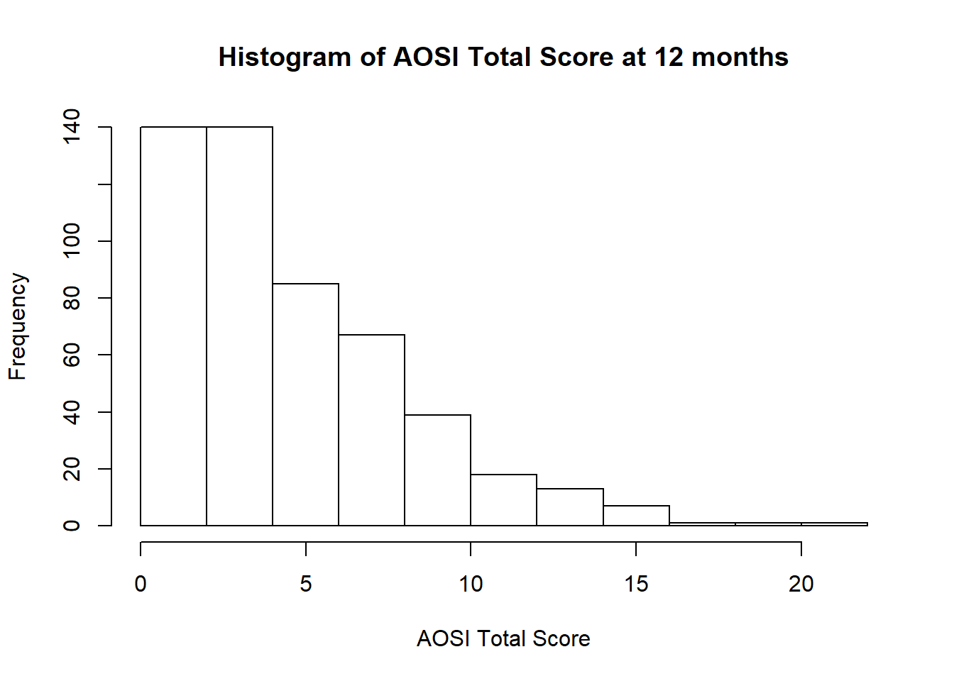
We can see that it is most likely that AOSI total score will be between 0 and 10, with values higher then 10 unlikely. This type of distribution is called skewed, specifically right skewed as it has a long “tail” to the right and most of the probability to the left. A left skewed distribution is the opposite. We can also consider the distribution of our variable \(X\) conditional on value y of another variable Y. Conditional means “only on the population with Y=y”. This is referred to as the conditional distribution of \(X\) for \(Y=y\). For example, while we have created the histogram of AOSI total score for the entire sample, we may want to visualize the distribution of AOSI total score separately for each of the following diagnosis groups, High Risk: ASD, High Risk: Negative, and Low Risk: Negative. For example, we create the histogram for the High Risk: ASD group below.
data_HRASD <- data %>% filter(GROUP=="HR_ASD")
hist(data_HRASD$V12.aosi.total_score_1_18, xlab = "AOSI Total Score",
main="Conditional Histogram of AOSI Total Score \nat 12 months for High Risk: ASD group") 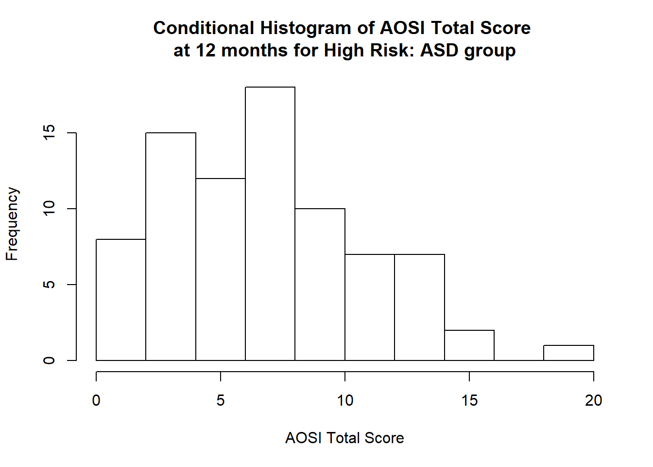
# can see variable is considered to be a string by default in the data; need to force it to be numeric to create a histogramStatistical analyses are often designed to estimate certain characteristics of a variable’s (or many variables’) distribution. These characteristics are usually referred to as parameters. Often times, these parameters are the mean, variance, median/quantiles, or probabilities of specific values (for a discrete variable, i.e., probability of positive ASD diagnosis). We do not know the true values of these parameters, so we try to obtain an accurate approximation of them based on random samples (your data) from the distribution/population of interest. These approximations will vary from sample to sample due to the randomness behind the selection of these samples and their finite size. Thus, we also need to account for the variance of these approximations when completing our analyses. This analysis, composed of the estimation of the parameters as well as accounting for the variance of this estimation, is referred to statistical inference.
7.2.1 Parameter Estimation: Mean, Median, tutorial, Quantiles
Here, we discuss the estimation of specific parameters that are usually of interest for continuous variables. For categorical variables, see Chapter 6. These parameters are the mean, median, variance, and quantiles. Often, you will see these estimates summarized in “Table 1” in research articles. To see how to create such summaries, see the Chapter 9. Here, we discuss the methodology behind their estimation as well as how to compute these estimates in R.
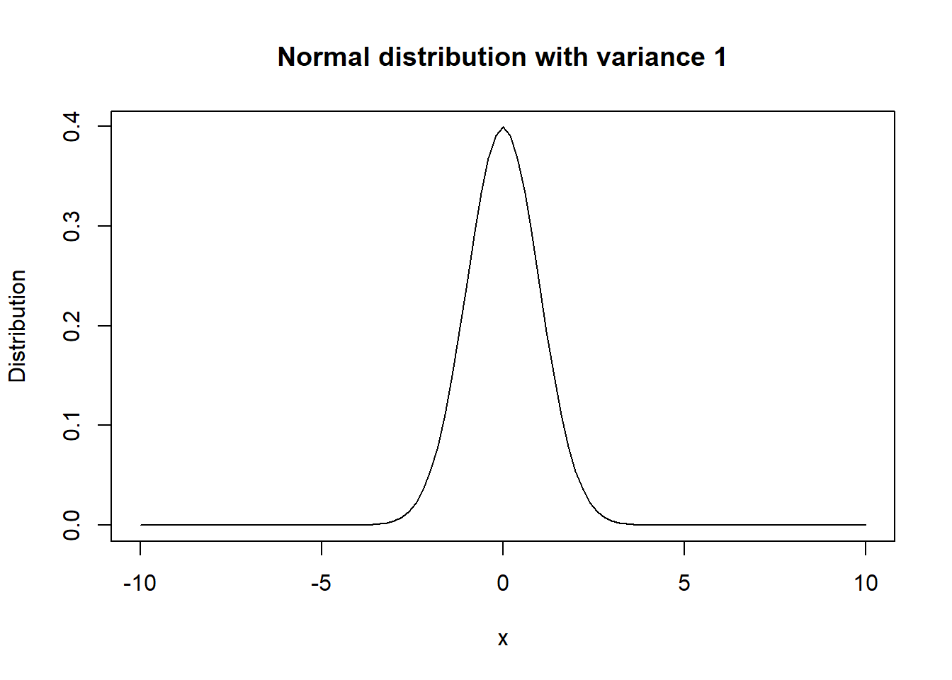
Both the mean and median can intuitively be thought of as measures of the “center” of the distribution. The variance can be thought of a measure of the “spread” of the distribution. To illustrate variance, we plot two normal distributions both with mean 0 but one with a variance of 1 and another a variance of 4. The increase in the likely range of values with a variance of 4 is quite evident, and the probabilities are more spread out. Note that the standard deviation is just the square root of the variance.
We estimate the distribution’s mean, median, variance, and quantiles using the usual sample mean, median, variance, and quantiles respectively. These can be calculated in R using the functions mean(), median(), var(), and quantile() respectively. Note: when using quantile(), the minimum and maximum values in the sample are also provided. We illustrate these functions below using AOSI total score at 12 months. Also, note the inclusion of na.rm=TRUE into these functions. By default, when calculating these estimates, if a missing value is encountered, R outputs NA (missing). Thus, we need to tell R to remove these missing values before computing the estimates.
mean(data$V12.aosi.total_score_1_18, na.rm=TRUE)## [1] 4.980469var(data$V12.aosi.total_score_1_18, na.rm=TRUE)## [1] 13.08377median(data$V12.aosi.total_score_1_18, na.rm=TRUE)## [1] 4quantile(data$V12.aosi.total_score_1_18, na.rm=TRUE)## 0% 25% 50% 75% 100%
## 0 2 4 7 22However, we often want to see these estimates (and others) for many variables in our dataset without having to calculate each one separately. This can be done using summary(). These estimates are often referred to as summary statistics of the data. We compute summary statistics for a number of the variables in the dataset below.
data_small <- data %>%
  select(V12.aosi.total_score_1_18, V06.aosi.total_score_1_18,
         V12.aosi.Candidate_Age)
summary(data_small)
## V12.aosi.total_score_1_18 V06.aosi.total_score_1_18
## Min. : 0.00 Min. : 1.000
## 1st Qu.: 2.00 1st Qu.: 7.000
## Median : 4.00 Median : 9.000
## Mean : 4.98 Mean : 9.562
## 3rd Qu.: 7.00 3rd Qu.:12.000
## Max. :22.00 Max. :28.000
## NA's :75 NA's :105
## V12.aosi.Candidate_Age
## Min. : 0.00
## 1st Qu.:12.20
## Median :12.50
## Mean :12.59
## 3rd Qu.:12.90
## Max. :16.70
## NA's :75There are also a number of packages which expand R’s functionality in computing these summary statistics. One recommended package is the Hmisc package. It includes the function describe() which is an improved version of of summary(); describe() is used below with the same variables.
library(Hmisc)
describe(data_small)
## data_small
##
## 3 Variables 587 Observations
## ---------------------------------------------------------------------------
## V12.aosi.total_score_1_18
## n missing distinct Info Mean Gmd .05 .10
## 512 75 20 0.99 4.98 3.901 1 1
## .25 .50 .75 .90 .95
## 2 4 7 10 12
##
## Value 0 1 2 3 4 5 6 7 8 9
## Frequency 23 51 66 68 72 51 34 40 27 18
## Proportion 0.045 0.100 0.129 0.133 0.141 0.100 0.066 0.078 0.053 0.035
##
## Value 10 11 12 13 14 15 16 17 20 22
## Frequency 21 10 8 7 6 4 3 1 1 1
## Proportion 0.041 0.020 0.016 0.014 0.012 0.008 0.006 0.002 0.002 0.002
## ---------------------------------------------------------------------------
## V06.aosi.total_score_1_18
## n missing distinct Info Mean Gmd .05 .10
## 482 105 24 0.994 9.562 4.622 4 5
## .25 .50 .75 .90 .95
## 7 9 12 15 17
##
## lowest : 1 2 3 4 5, highest: 20 21 22 24 28
## ---------------------------------------------------------------------------
## V12.aosi.Candidate_Age
## n missing distinct Info Mean Gmd .05 .10
## 512 75 37 0.994 12.59 0.7036 11.9 12.0
## .25 .50 .75 .90 .95
## 12.2 12.5 12.9 13.4 13.9
##
## lowest : 0.0 11.4 11.6 11.7 11.8, highest: 14.9 15.1 15.6 15.9 16.7
## ---------------------------------------------------------------------------7.2.2 Accounting for estimation variance and hypothesis testing
While these estimates provide approximations to the parameters of interest, they 1) have some degree of error and 2) vary from sample to sample. To illustrate this, 5 simulated datasets, each of size 100 and with a single variable are generated under a mean of 0. The sample mean is calculated for each of these 5 samples. We see that 1) these sample means differ across the samples and 2) none are exactly 0. Thus, we need to account for this variance when providing the approximations.
data_sim <- list()
for(i in 1:5){
  data_sim[[i]] <- rnorm(100, 0, 1)
}

lapply(data_sim, mean)
## [[1]]
## [1] 0.01816081
##
## [[2]]
## [1] -0.1085414
##
## [[3]]
## [1] -0.04594208
##
## [[4]]
## [1] -0.06228348
##
## [[5]]
## [1] -0.18206037.2.3 Confidence intervals
This is generally done by including a confidence interval with your approximation, more specially a \(x\)% confidence interval where \(x\) is some number between 0 and 100. Intuitively, you can interpret a confidence interval as a “reasonable” range of values for your parameter of interest based on your data. Increasing the percentage of the confidence interval increases its width, and thus increases the chances that the confidence interval from a sample will contain the true parameter. However, this increasing width also decreases the precision of the information you receive from the confidence interval, so there is a trade off. Generally, 95% is used (though this is just convention).
As an example, we considering computing a confidence interval for the mean. Consider AOSI total score at 12 months from our dataset. We have already computed an estimate of the mean; let us add a confidence interval to this estimate. This can be done using the t.test() function (which has other uses which we cover later).
t.test(data$V12.aosi.total_score_1_18)##
## One Sample t-test
##
## data: data$V12.aosi.total_score_1_18
## t = 31.156, df = 511, p-value < 2.2e-16
## alternative hypothesis: true mean is not equal to 0
## 95 percent confidence interval:
## 4.666411 5.294526
## sample estimates:
## mean of x
## 4.980469Let us focus on the bottom of the output for now; we cover the top later. We see that we approximate that the mean AOSI total score at 12 months in the population is 4.98 and a reasonable set of values for this mean in the population is 4.67 to 5.29 using a 95% confidence interval.
7.2.4 Hypothesis testing
In order to come to a conclusion about a paramater from the sample information, hypothesis testing is generally used.
The setup is the following: suppose we are interested in inferring if the mean for a variable is some value, say \(\mu_0\). From the data we have, we would like to make an educated guess about the claim that the mean is \(\mu_0\). The main principle in scientific research is that one makes a claim or hypothesis, conducts an experiment, and sees if the results of the experiment contradict the claim. This is the same reasoning that governs hypothesis testing.
To start, we make a claim which we would “like” to refute (for example, a treatment has no effect). This claim is referred to as the null hypothesis. For example, consider the null hypothesis that the mean is \(\mu_0\). We then define the contradiction to this claim, that the mean is NOT \(\mu_0\), as the alternative hypothesis. Finally, we take the information from our data, and see if there is enough evidence to reject the null hypothesis in favor of the alternative. If there is not enough evidence, then we fail to reject the null. That is, we never accept the null or prove that the null is true. Recall that the null is our baseline claim that we are aiming to refute; if we accepted the null, then we would be “proving true” that which we initially claimed to hold.
How do we determine if we have “enough evidence” to reject the null? The following process is generally used. First, we reduce our data down to a single value that is related to the hypothesis being tested. This value is called a test statistic. Then, we see how much the observed test statistic from our data deviates from the range of values we would expect if the null hypothesis were true. If this deivation is large enough, we decide to reject the null. Otherwise, we fail to reject.
This is best explained by example. Consider our null hypothesis of the mean is \(\mu_0\). Intuitively, we would calculate the sample mean and use it as our test statistic, and compare its value to \(\mu_0\). If the sample mean is “close” to \(\mu_0\), we would fail to reject, otherwise we would reject. For example, recall that for AOSI total score at 12 months, the sample mean ws 4.98. For our null hypothesis was that the population mean was \(\mu_0\)=5, we probably would not have enough evidence reject the null. However, we need a formal way of measuring the deviation from the null, preferrably one that is independent of the variable’s units. The p-value serves as this measure.
Formally, the p-value measures the probability of seeing a test statistic value that is as extreme or more extreme from the null hypothesis then the test statistic value you actually observed. Informally, you can think of a p-value as a unit agnostic measure of how much your data deivates from the null hypothesis. We calculate the p-value using the observed value of the test statistic as well as the test statistic’s distribution (also referred to as its sampling distribution); this distribution is how we are able to compute the probablity which the p-value reflects.
To conduct the hypothesis test corresponding to the null hypothesis that the population mean is 0, a one sample t-test is often used. We will cover this in more detail later; here we use it to illustrate the above concepts. The t.test() function can also be used to conduct this hypothesis test. We consider testing if the mean AOSI total score at 12 months is 0. Note that we can choose a values different from 0 to use in our null hypothesis by adding the argument mu=x, where x is the value of interest.
t.test(data$V12.aosi.total_score_1_18)##
## One Sample t-test
##
## data: data$V12.aosi.total_score_1_18
## t = 31.156, df = 511, p-value < 2.2e-16
## alternative hypothesis: true mean is not equal to 0
## 95 percent confidence interval:
## 4.666411 5.294526
## sample estimates:
## mean of x
## 4.980469The top part of the output contains the hypothesis test results. We see that the test statistic (denoted by t) is 31.156 and the corresponding p-value is essentially 0. Note that there is a one to one correspondence between the test statistic value and the p-value. Thus, reporting the p-value only is sufficient. We see that the p-value is very small; a small p-value implies that the data deviates from the null. However, to make a reject or fail to reject decision, we have to set a threshold for this p-value. Generally, people select 0.05 as a threshold; below 0.05 implies the evidence is strong enough to reject and above 0.05 implies the evidence is not strong enough. However this is just a rule of thumb and one could justify a different threshold.
Furthermore, it may not be wise to make an all or nothing decision in terms of judging the scientific value of the results. Using a p-value threshold implies that a p-value of 0.051 has the same interpretation as a p-vale of 0.51 and that a p-value of 0.049 is “significant” evidence while a p-value of 0.051 is not. This dramatically limits the scientific information that the results are providing. Instead, it is better to interpret p-values more broadly and in terms of their strength of evidence. For example, a p-value of 0.06 or 0.025 may indicate “strong evidence” in favor of the alternative hypothesis and 0.10 or 0.12 may indicate “moderate evidence”. Simply reducing the interpretation to “significant” or “not significant” is not optimal and should be avoided.
7.2.5 Hypothesis Testing with Means
Here we cover methods to conduct hypothesis testing with population means. You will likely recognize many of these methods; we cover t-tests and ANOVA. We illustrate these using AOSI total score at 12 months and diagnosis group (High Risk: ASD, High Risk: Negative, Low Risk: Negative)
7.2.5.1 T-tests: One Sample and Two Sample
First, consider testing the null hypothesis that the mean AOSI total score at 12 months is 0 in the population. As discussed before, this comparison of a single mean to a value is generally done with a one sample t-test. Recall that anytime we do a hypothesis test, we require the following: 1) Test statistic 2) Distribution of the test statistic 3) P-value from this distribution and the test statistic’s observed value
In this case, the test statistic is denoted by \(T\) since it has a \(T\) distribution. This test statistic \(T\) is equal to the sample mean minus the null value (often 0) and then divided by the spread of the sample mean (called standard error). \(T\) distributions are differentiated by the parameter called degrees of freedom (similar to how normal distributions are differentiated by their mean and variance). Using the value of \(T\) with the value of the degrees of freedom and the \(T\) distribution, components 1) and 2), we can calculate a p-value. All three of these components are provided in the output from t.test(), along with the alternative hypothesis of the test (that the mean is not 0).
t.test(data$V12.aosi.total_score_1_18)##
## One Sample t-test
##
## data: data$V12.aosi.total_score_1_18
## t = 31.156, df = 511, p-value < 2.2e-16
## alternative hypothesis: true mean is not equal to 0
## 95 percent confidence interval:
## 4.666411 5.294526
## sample estimates:
## mean of x
## 4.980469We see that under a p-value of about 0, we have strong evidence in favor of the mean AOSI total score at 12 months not equalling 0. Note that you can also see that 0 is quite outside the 95% confidence interval, indicating that 0 is not a reasonable value for the population mean based on this dataset (which points to the alternative hypothesis). It turns out that p-values and confidence intervals are generally linked together and will agree in this fashion by their design.
Note that for this process to be valid, some assumptions are made. They are a) AOSI total score at 12 months is normally distributed and b) all observations are independent. If one or more of these is violated, the results from your one-sample t-test will be invalid.
Now suppose we wanted to compare mean AOSI total score at 12 months between two diagnosis groups, such as High Risk: ASD and High Risk: Negative. Specifically, the null hypothesis will be that the means are the same between the two groups. The common corresponding test is called a two sample t-test. Again, we use the function t.test(). Here, we use y~x notation where x is the grouping variable to do the two sample test. You will again obtain a test statistic t, degrees of freedom, and a p-value. As in the one sample case, this test statistic also has a \(T\) distribution.
data_HR <- data %>%
  filter(GROUP=="HR_ASD"|GROUP=="HR_neg")

t.test(V12.aosi.total_score_1_18~GROUP,data=data_HR)
##
## Welch Two Sample t-test
##
## data: V12.aosi.total_score_1_18 by GROUP
## t = 4.9977, df = 113.84, p-value = 2.119e-06
## alternative hypothesis: true difference in means is not equal to 0
## 95 percent confidence interval:
## 1.506931 3.486090
## sample estimates:
## mean in group HR_ASD mean in group HR_neg
## 7.337500 4.840989You can see R provides the following, starting from the top. 1) Test statistic t, degrees of freedom, and p-value 2) alternative hypothesis 3) 95% confidence interval for the difference in the means 4) sample means for each group
We see that, as expected, based on a p-value about 0, we have strong evidence that the mean AOSI total scores at 12 months are different between High Risk: ASD and High Risk: Negative. This can also be seen in 0 being far away from the confidence interval and the sample means of 7.34 and 4.84 being quite different from one another.
7.2.5.2 ANOVA
Suppose we want to compare more then two groups’ means. For example, suppose we want to compare the mean AOSI total score at 12 months for the High Risk: ASD, High Risk: Negative, and Low Risk: Negative groups. This is done using an ANOVA F test. The null hypothesis is that the mean AOSI total score at 12 months is same in all three groups. The alternative is that at least one group’s mean differs from the rest. We can conduct this test in R using aov(). Again, it uses formula notation (y~x). We conduct this test below. Note that many components are calculated by R for this test. To obtain the main values of interest, we must save the output as an object (which stores all of the components) and then use the function summary() on this object.
aov_object <- aov(V12.aosi.total_score_1_18~GROUP, data=data)
summary(aov_object)
## Df Sum Sq Mean Sq F value Pr(>F)
## GROUP 3 599 199.81 16.68 2.39e-10 ***
## Residuals 508 6086 11.98
## ---
## Signif. codes: 0 '***' 0.001 '**' 0.01 '*' 0.05 '.' 0.1 ' ' 1
## 75 observations deleted due to missingnessWe see degrees of freedom are provided (3 and 508 in this example), the value of the test statistic (F value=16.68) and the corresponding p-value (2.39e-10 or essentially 0). For an ANOVA F test, the test statistic \(F\) has an \(F\) distribution. An \(F\) distribution is defined by two degrees of freedom parameters. Using this F statistic value and F distribution, the p-value can be calculated.
While an ANOVA F test will infer if the groups differ overall, we would like to see which groups differ. This generally done by doing all of the pairwise comparisons. For our example, that would entail hypothesis tests for 1) HR: ASD vs HR: Negative, 2) HR: ASD vs LR: Negative, 3) HR: Negative vs LR: Negative, etc. for 6 total tests. Recall when comparing two groups’ means, we can use a two sample t-test. For each pairwise test, we use this two sample t-test. Then, we interpret the test results for each pair separately. This is frequently referred to as post-hoc analysis. It turns out that because we are conducting multiple hypothesis tests at once, we need to “correct” each p-value from these pairwise comparisons to account for this multiple comparison. Why this is the case is beyond the scope of these tutorials. Generally, the correction done is called Tukey’s Method, though other corrections such as Bonferroni or Holm’s Method can also be used. These corrected p-values can then be “validly” interpreted like usual p-values. To compute this post-hoc analysis in R using Tukey’s Method, use the function TukeyASD() with the object from aov().
TukeyHSD(aov_object)## Tukey multiple comparisons of means
## 95% family-wise confidence level
##
## Fit: aov(formula = V12.aosi.total_score_1_18 ~ GROUP, data = data)
##
## $GROUP
## diff lwr upr p adj
## HR_neg-HR_ASD -2.4965106 -3.626229 -1.36679183 0.0000001
## LR_ASD-HR_ASD -3.6708333 -8.917563 1.57589610 0.2728961
## LR_neg-HR_ASD -3.3511986 -4.592245 -2.11015217 0.0000000
## LR_ASD-HR_neg -1.1743227 -6.352589 4.00394397 0.9367305
## LR_neg-HR_neg -0.8546880 -1.763793 0.05441738 0.0740168
## LR_neg-LR_ASD 0.3196347 -4.884054 5.52332358 0.9985859The output contains the following: 1) Difference in sample means between the groups (diff) 2) 95% confidence intervals for each mean difference (lwr and upr) 3) Corrected p-values for each pairwise comparison (p adj)
This entire ANOVA analysis provides valid results under the following assumptions 1) All groups’ values are normally distributed with the same variance 2) All observations are independent (both within the groups and between the groups)
The first assumption can be checked visually using a histogram and by estimating the variances with confidence intervals, or conducting hypothesis tests for equal variances (not covered here). The second assumption is verified based on the study from which the data originated.