3 Objects and Functions
3.1 Intro
Data processing and analysis in R essentially boils due to creating output and saving that output, either temporarily to use later in your analysis or permanently onto your computer’s hard drive for later reference or to share with others. In R, output is created using commands called and when saving output temporarily to be used later in your R session, the output is saved as an .
For example, suppose you have a previously saved Excel dataset you wish to analyze by performing linear regression. First, you must load this Excel dataset into R, which is done using a function. However, you want to give this read-in dataset a name so that you easily reference it in your R session. Thus, you save the read-in dataset as an R object called excel_data. Then, you use another function on excel_data to run the linear regression, whose results you store as another object called fit_results to be easily accessible in your R session. Note that objects excel_data and fit_results are not stored permanently on your computer but are instead stored on the computer’s RAM. Thus, when your computer is restarted, these R objects will be deleted (though the Excel file itself is a permanent file on your computer: the form of the Excel dataset created when read-in by R is not permanent). A similar example is detailed in the following code using an IBIS dataset, where a linear regression model is fit where the outcome is AOSI Total Score at Month 12 and the independent variable is Age at Month 12.
## Read-in Excel dataset using function called read.csv
read.csv("Data/cross-sec_aosi.csv") # look at the console: running command reads-in data, however data is not saved; cannot reference dataset using name since we have only read it in, not given it a name/saved it in R

excel_data <- read.csv("Data/cross-sec_aosi.csv",
                       na.strings = c(".", "", " ")) # are telling R to take output from function read.csv (the read-in data) and save it as object excel_data

# Can see dataset no longer pops up in console: when storing output as object, R does not print the output for you

excel_data # running just the object is a command: tells R to print out the output stored in the object. Now can easily reference dataset set using excel_data
## Run linear regression using ASOSI Total Score as outcome, Diagnosis as predictor variable. Running regression models is discussed in detailed in Chapter 8
lm(V12.aosi.total_score_1_18~V12.aosi.Candidate_Age, data=excel_data) # using AOSI at month 12##
## Call:
## lm(formula = V12.aosi.total_score_1_18 ~ V12.aosi.Candidate_Age,
## data = excel_data)
##
## Coefficients:
## (Intercept) V12.aosi.Candidate_Age
## 3.98890 0.07879You can see that the end result is the estimated intercept and slope from your linear regression model. By the end of all of these tutorials, you will understand every step of the above code. By the end of this tutorial, you should be able to understand the above code in general as a series of functions and objects.
3.2 Functions
Every time R is given a command, R produces the output specified from the command. As a simple example, suppose you wish to add 2 and 2.
2+2## [1] 4After running the above line of code, you will see R output the result of the addition in the console. The command + is called a function (specifically an operation, a class of commands/functions). For usability, mathematical operators such as +,-,/, and * have this form, although most functions have the following form: fun(x,y,z)
where fun is the name of the function, and x,y, and z are options the user places in the function which modify how it operates. These options are called arguments. This example function has 3 arguments (x,y,z), however functions can have many more arguments for the user to manipulate. Note that all functions have default values for most of their arguments which will automatically be used without the user having to specify them.
As a more interesting example, suppose you want to read-in some data into R which you will analyze. The dataset is of a sample of children from IBIS, and includes site, geneder, and AOSI information at month 6 and month 12 visit. The dataset is found in the file cross-sec_aosi.csv. To do read this file in, we must choose the right function so R knows what we want it to do. A function that will do this command is read.csv(). This function has default values for all of its arguments, except for the first one where you much specify the file path of CSV dataset you want to read-in. First, let’s leave the default values as is and read-in the data.
read.csv("Data/cross-sec_aosi.csv")From the previous tutorial, since the file is in our working directory, we only need to specify the file name and not the whole path. Notice that the file path needs to be in quotes (use of quotes will be discussed later in this chapter). After you run the code, you will notice the dataset is printed in the R console. For reading in other files types, different functions are needed. Many of these are found in the package haven which includes functions such as read_sas() for SAS files and read_spss() for SPSS files.
When learning and using functions it is useful to submit the command ?fun where fun is the name of the chosen function. For example, try running ?read.csv in your script.
# ?read.csvYou will see in the lower right-hand window, the Help tab will open up along with a description of the function read.csv(), including all of its arguments, some notes about the function and its usage, and some examples to refer to.
However, this is not a visually pleasing way to view the data. Furthermore, this dataset has not be given a name in R to reference, which will make using this data difficult to use in your R script All R has done is read-in the CSV data, converted it into a format it understands, and then printed this output. Actually storing this output in R and giving it a name so that it can be easily referenced later involves creating objects.
3.3 Objects
Output generated in R can be temporarily saved in your R session with a name to be referenced later. This saved output is called an object. The most intuitive example is reading in data to be analyzed. Let’s read-in the previous Excel sheet and save it as an object named excel_data. To save output as an object with a name, the command is
name <- fun(…)
excel_data <- read.csv("Data/cross-sec_aosi.csv")Now the dataset can be easily accessed by using excel_data in your code. For example, one way of intuitively viewing data in your R session is using the function View() (note: case matters in R).
3.4 Object classes and types
Now that objects have been introduced, we will go into further detail about them which will be vital when using functions and understanding errors. While you can use R without understanding this section, learning this information will help you understand the structure of R which is essential when using R on real data.
Every object in R is classified into a class and a type. The object’s class represents the general structure of the object as a whole, while the type is a more specific description of the actual contents of the object. These concepts are best explained with examples.
The classes that you will see likely see in practice are a vector, matrix, list, and data frame. The types you will see in pratice are numeric, character (letters/words), factor (group levels), and logical (TRUE/T or FALSE/F). Numeric means the values are interpreted as numbers. Character type refers to values which are “strings” (combinations) of letters, words, symbols, numbers, etc. surrounded by quotation marks. Factor types are explained later in this chapter. The values TRUE and FALSE (caps required, no quotations) have a specific meaning in R, and objects with these values are referred to as logical types (these are not character types, values not surrounded by quotes). For all types, the value NA (caps required, no quotes) is interpreted by R as a missing value; NA is the only value in R which refers to a missing value.
3.4.1 Vectors
A vector is a single-dimension collection of values, all of which must have the same type. For example, (0,1,2,3) is a numeric vector of length 4, and (“Yes”, “No”, “Maybe”) is a character vector of length 3. When working with a dataset, each row can be considered as a vector as can each column. As with all objects, these vectors can be created and saved with a name in R. This is done using c(…) where the elements of the vector are place inside () separated by commas. Some examples are found below. You can think of a vector as either a variable (column) in your dataset or an observation (row) in your dataset. To index vectors, use [] where the indicies of interest are placed inside the []; see below for an example. One function of use with vectors is length(), which will output the number of values in the vector.
c(0,1,2,3) # outputs as vector## [1] 0 1 2 3c("Yes", "No", "Maybe")## [1] "Yes" "No" "Maybe"num_vect <- c(0,1,2,3) # save vector as named object
char_vect <- c("Yes", "No", "Maybe")
num_vect # outputs saved vector in console## [1] 0 1 2 3char_vect## [1] "Yes" "No" "Maybe"num_vect[1:3] # a:b creates sequence of integers from a to b## [1] 0 1 2char_vect[c(1,2)] # selecting the 1st and 2nd entries## [1] "Yes" "No"char_vect[1,2] # Creates an error; need to have single entity inside []## Error in char_vect[1, 2]: incorrect number of dimensionslength(num_vect) # length=3, vector has 3 elements## [1] 43.4.2 Matricies
A matrix is a two-dimensional collection of values, all of which need to be the same type. When viewing a matrix in R, it largely looks like an Excel spreadsheet. In standard data analysis, matricies are rarely used so they are not covered here in much detail. An example of a matrix is shown below; they can created using the matrix() function, though you will rarely if ever create matricies in standard data analysis. It is more important to know how to manipulate them, which is discussed in a later section of this chapter. Notice that although numbers 1,2,3 were specified as entries, these show up as “1”,“2”, and “3” (characters) respectively in the outputted matrix. This called coercion, where R forces values into a certain type to meet the requires of the class of the object. It is important to recognize when coercion happens and why, since some commands only work on specific types of values (for example when taking the mean of a variable in your dataset, the values need to be numeric).
matrix(c(1,2,3,"Yes", "No", "Maybe"), nrow=3, ncol=2) # numbers forced into characters to match type with the non-numeric entries of the matrix## [,1] [,2]
## [1,] "1" "Yes"
## [2,] "2" "No"
## [3,] "3" "Maybe"You can also combine multiple vectors into a matrix, either row-wise or column-wise. This is done using the rbind() and cbind() functions respectively.
nums <- c(1,2,3) # create numeric vector
words <- c("Yes", "No", "Maybe")

# notice since the vectors were saved as objects before binding, the names show up as names for the rows for rbind and columns for cbind respectively.  In a matrix, the rows and/or cols can be given names as shown here
rbind(nums, words)
## [,1] [,2] [,3]
## nums "1" "2" "3"
## words "Yes" "No" "Maybe"cbind(nums, words)## nums words
## [1,] "1" "Yes"
## [2,] "2" "No"
## [3,] "3" "Maybe"3.4.3 Lists
Recall the two above classes required all elements be of the same type; for example, you cannot have both number and character values in the object. Lists allow values to be of different types. Essentially, a list of a collection of other objects. Generally, lists will be a collection of different vectors and/or matricies. For example, your list could be composed of 2 vectors, one of which with numeric values and the other with character values. Any combination of vectors and/or matricies is allowed, along with many other possibilities (including a list composed of multiple lists). Lists are created using the list() function, as shown in the following example.
nums <- c(1,2,3) # create numeric vector
words <- c("Yes", "No", "Maybe") # create character
# store the 2 vectors together as a list
list(nums, words) ## [[1]]
## [1] 1 2 3
##
## [[2]]
## [1] "Yes" "No" "Maybe"Each element of the list is indexed by [[]]; in the above example, you can see the 2 vectors used to create the list. Notice the numeric vector does not have quotes surrounding it; within the list, the vector is still considered numeric as desired. Lists are useful since they allow you to hold objects that are of different classes together in a single entity, making them easier to keep track of and reference later. You will see lists come up very frequently when using R for data analysis and it is important to become comfortable with them.
3.4.4 Data Frames
Generally, when you read-in data as an object, it will be stored in R as a data frame. Essentially, a data frame is a list of the individual columns/variables which compose the dataset, where the columns are considered vectors. That is, a data frame is a list of vectors, but when outputted is shown like a matrix with rows and columns instead of the usual look of a list. While data frames can be viewed in the console like all objects by just entering their name, it is most useful to see them using the View() function. Another useful function for data frames (and matricies) is dim(), which will output the number of observations (rows) and columns (variables) in your dataset. The function names() will output the column (variable) names of your dataset. This function can also be used in a similar way with vectors, matricies, and lists.
excel_data <- read.csv("Data/AOSI_small.csv") # read-in data as data frame, save as named object
excel_data # view dataset in console; hard to read especially for datasets of usual size## Identifiers GROUP Study_Site Gender V06.aosi.Candidate_Age
## 1 1 HR_ASD PHI Male 7.1
## 2 2 HR_ASD PHI Male 6.1
## 3 3 HR_ASD PHI Male 6.6
## 4 4 HR_ASD PHI Male .
## 5 5 HR_neg PHI Male 6.8
## 6 6 HR_neg PHI Male .
## 7 7 HR_ASD PHI Male 6.2
## 8 8 HR_ASD PHI Male 6.2
## 9 9 HR_neg PHI Male .
## 10 10 HR_ASD PHI Male .
## V06.aosi.total_score_1_18 V12.aosi.Candidate_Age
## 1 8 12.5
## 2 18 12.4
## 3 4 12.9
## 4 . 12.7
## 5 6 .
## 6 . 12.1
## 7 16 12.3
## 8 10 12.2
## 9 . 12.4
## 10 . 12.2
## V12.aosi.total_score_1_18
## 1 3
## 2 10
## 3 2
## 4 3
## 5 .
## 6 4
## 7 4
## 8 14
## 9 1
## 10 7# View(excel_data)
# can see dataset pops up in tab in upper right window, easy to see/scroll through
names(excel_data)## [1] "Identifiers" "GROUP"
## [3] "Study_Site" "Gender"
## [5] "V06.aosi.Candidate_Age" "V06.aosi.total_score_1_18"
## [7] "V12.aosi.Candidate_Age" "V12.aosi.total_score_1_18"dim(excel_data)## [1] 10 83.4.5 Types
Object types are a more intuitive idea and have been mentioned above; types describe the actual values inside the object. Recall the common types are character (letters/words), numeric, factor (group levels), and logical (TRUE/T or FALSE/F).
Recall that for vectors and matricies, all entries must be the same type. Thus, a vector/matrix with all numeric values is of type numeric, with all character values is of type character, with all logical vaues is of type logical, etc. Since lists and data frames of made of up a collection of vectors, matricies, and/or lists, they do not have an explicit “type”. To see what type an object is, you can use the function typeof(). Note that when a list or data frame is inputted into the function, “list” or “df” respectively is returned.
num_vect <- c(1,2,3,4)
char_vect <- c("a","b","c","d")
log_vect <- c(T, F, TRUE, FALSE)
typeof(num_vect)## [1] "double"typeof(char_vect)## [1] "character"typeof(log_vect)## [1] "logical"matrix_ex <- cbind(num_vect, char_vect, log_vect)
typeof(matrix_ex)## [1] "character"list_ex <- list(num_vect, char_vect, log_vect, matrix_ex)
list_ex## [[1]]
## [1] 1 2 3 4
##
## [[2]]
## [1] "a" "b" "c" "d"
##
## [[3]]
## [1] TRUE FALSE TRUE FALSE
##
## [[4]]
## num_vect char_vect log_vect
## [1,] "1" "a" "TRUE"
## [2,] "2" "b" "FALSE"
## [3,] "3" "c" "TRUE"
## [4,] "4" "d" "FALSE"typeof(list_ex) # returns "list"; lists have no single type such as numeric, character, etc.## [1] "list"The factor type requires some explanation. Most character variables you will work with indicate group membership; for example a gender variable recorded as “Male”, “Female”, or “Other” or a treatment variable recorded as “Treatment” or “Control”. We want to treat these as groups, not separate words/strings. This can be done using the factor type. Note for many functions were you want the variable to be treated as a factor, for example in linear regression, R will convert the character variable into an appropriate factor variable. If the variable is actually numeric but you want it to reflect group membership (for example a 0, 1 variable indicating treatment), you likely will have to convert it yourself.
A factor variable, i.e. a vector of type factor, has two parts: the vector of values as well as a vector indicating what the factor “levels” (essentially labels for the groups) are. For example, consider the following character variable indicating the genders in a set of observations.
# M is male, F is female, O is other
genders <- c("M", "F", "M", "M", "F", "F", "F", "O", "O")
genders # print character vector## [1] "M" "F" "M" "M" "F" "F" "F" "O" "O"Let’s convert this to a factor variable; by default, R will automatically set the factor levels to the unique values in the variable (M, F, and O in this case). This is done using the factor() function. To see the levels assigned to a factor variable, use the function levels().
# M is male, F is female, O is other
genders_fact <- factor(genders)
genders_fact## [1] M F M M F F F O O
## Levels: F M Olevels(genders_fact)## [1] "F" "M" "O"To alter the levels, you overwrite the levels() output as seen below. Since the levels of a factor variable are actually a R object, you edit them by overwriting this object which is accessed using the levels() function. We overwrite the levels object by specifying a new character vector to define the levels; can see from the levels() call that they are saved as a character vector. After the levels are changed, you will see these changes also occur in the variable values. Note that you can also convert back to a character/numeric variable by using the as.character()/as.numeric() functions respectively.
# Original variable, levels
genders_fact## [1] M F M M F F F O O
## Levels: F M Olevels(genders_fact)## [1] "F" "M" "O"# Overwrite levels
levels(genders_fact) <- c("Female", "Male", "Other") # pay attention to order of levels, need to follow order as F->Female, M->Male, O->Other.
# New variable, levels
genders_fact## [1] Male Female Male Male Female Female Female Other Other
## Levels: Female Male Otherlevels(genders_fact)## [1] "Female" "Male" "Other"# convert back to character
as.character(genders_fact)## [1] "Male" "Female" "Male" "Male" "Female" "Female" "Female" "Other"
## [9] "Other"# Can also do numeric levels
levels(genders_fact) <- c(1, 0, 2)
genders_fact## [1] 0 1 0 0 1 1 1 2 2
## Levels: 1 0 2# convert to numeric
as.numeric(genders_fact)## [1] 2 1 2 2 1 1 1 3 3Most of the time in standard data analysis, you won’t have to manually convert variables to factor variables. When reading-in a dataset, you can have R automatically convert character variables to factors (will be covered in the next Chapter). When doing regression, R will automatically convert character variables to factors as well. However, for completeness and to understand certain errors which may occur when using R, it is useful to understand what factors are.
Understanding types is very important for using R. Certain functions only work on specific types; for example, you cannot compute the mean of a variable of character values. This concept will help you understand some errors that may come up.
3.5 Subsetting
Often times you will need to select specific parts of an object to view or using in your analysis; for example, computing the mean of a specific variable in your dataset or viewing only specific observations in your dataset based on some chosen critieria. In these tutorials, this is referred to as subsetting. There are 2 main ways to subset objects in R: 1) using Base R functions and 2) using functions from the dplyr package. Base R refers to the functions built into R by default; i.e., functions that do not require a package to be installed in order to access. You will likely use the dplyr method most of the time. However, for completeness and since the Base R method is useful to understand how R operates, it is important that you understand both.
3.6 Base R
The tools for subsetting in Base R differ depending on what class your object is. These tutorials cover the classes discussed previously: vectors, matricies, lists, and data frames. In general, for object x of any class, subsetting is done using x[…], where the values placed inside [] will determine how the object is subset. Note that when subsetting, you are not changing the original object x, but are creating a new object which is a “subset”" of x.
First, let’s discuss this operation for vectors. Recall vectors are single-dimension collections of values of the same type, for example x=(1,2,3,4). Vectors are subset by stating the indicies you either want to select or omit inside the []. Suppose we wanted to keep 1 from the vector (1,2,3,4). Since this is the 1st value in the vector by order from left to right, we would use x[1]. If we want to keep all values except 1, i.e. (2,3,4), we would use x[-1]; adding a negative to an index removes its value. If you want to select multiple indicies to include or remove, for example (2,3), you must use x[c(2,3)]. That is, you have provide these indices as a vector inside the []; R does not understand what 2,3 is unless represented as a vector. See below for some examples of this subsetting in action.
num <- c(2,4,6,8,10)
char <- c('a','e','i','o','u')
num[1]## [1] 2num[-4]## [1] 2 4 6 10num[c(1,3)] # correct## [1] 2 6num[1:3] # 1:3 is interpretated in R as c(1,2,3), this notation is useful as a shortcut when selecting many values## [1] 2 4 6char[1]## [1] "a"char[-4]## [1] "a" "e" "i" "u"char[c(1,3)] # correct## [1] "a" "i"char[1:3] # 1:3 is interpretated in R as c(1,2,3), this notation is useful as a shortcut when selecting many values## [1] "a" "e" "i"# num[c(1,-2)] # cannot mix positive and negative indicies, running line will give error
# char[c(1,-2)] # cannot mix positive and negative indicies, running line will give errorSecond, let’s discuss matricies. Working with matricies is similar to working with vectors, the main difference being you can select indicies for two dimensions (rows and columns) instead of just one. Suppose x is a matrix. Then we can subset x using x[,] where row indicies go to the left of the comma and column indicies go to the right. To select all rows/columns leave the right/left side empty respectively. The rules for selecting indicies are the same as before: use a vector when selecting multiple indicies, use negative indicies to omit a row/column, and do not mix positive and negative indicies. If your matrix’s columns are named, you can also refer to these names inside [] as strings instead of referring to the index of the column. See below for some examples.
nums <- c(1,2,3) # create numeric vector
words <- c("Yes", "No", "Maybe")
logs <- c(TRUE, FALSE, TRUE)
matrix <- cbind(nums, words, logs)
matrix[,c("nums","words")] # select words and nums columns using strings, as this matrix has column names## nums words
## [1,] "1" "Yes"
## [2,] "2" "No"
## [3,] "3" "Maybe"matrix[,c(1,2)] # select words and nums columns by indicies## nums words
## [1,] "1" "Yes"
## [2,] "2" "No"
## [3,] "3" "Maybe"matrix[1,c("nums","words")] # select words and nums columns, select only 1st row## nums words
## "1" "Yes"Third, let’s discuss lists. Recall lists of collections of other objects, such as vectors, matricies, or other lists. Lists introduce [[]] as subset operator, used to select the specific objects in the collection. You can think of [[]] as selecting “outer” elements, and then using [] to subset these outer elements. You will seldom be subsetting lists, and generally will using be using [[]] when you do subset them.
Another way to subset lists instead of [[]] is using $. Suppose you have a list x which contains two objects with the names x_1 and x_2 respectively. Then to select the first object, you either using x[[1]] from before or using x$x_1, or using x[[“x_1”]]. This will be referred to again next when we discuss data frames. Some examples are provided below.
nums <- c(1,2,3) # create numeric vector
words <- c("Yes", "No", "Maybe")
logs <- c(TRUE, FALSE, TRUE)
matrix <- cbind(nums, words)
example_lst <- list(matrix, logs) # create a list containing a matrix and vector, without names
example_lst # notice the [[]] indexing each part of the list## [[1]]
##      nums words
## [1,] "1"  "Yes"
## [2,] "2"  "No"
## [3,] "3"  "Maybe"
##
## [[2]]
## [1] TRUE FALSE TRUEexample_lst <- list(x_1=matrix, x_2=logs) # create a list containing a matrix and vector, with names x_1 and x_2 respectively
example_lst # notice the [[]] indicies have been replaced with their specified names## $x_1
##      nums words
## [1,] "1"  "Yes"
## [2,] "2"  "No"
## [3,] "3"  "Maybe"
##
## $x_2
## [1] TRUE FALSE TRUEexample_lst[[1]] # selects the matrix from the list, its first element## nums words
## [1,] "1" "Yes"
## [2,] "2" "No"
## [3,] "3" "Maybe"example_lst$x_1 # also selects the matrix## nums words
## [1,] "1" "Yes"
## [2,] "2" "No"
## [3,] "3" "Maybe"example_lst[[2]] # selects the vector## [1] TRUE FALSE TRUEexample_lst[[2]][c(1,2)] # after selecting the vector, we can subset the vector using [] as discussed earlier## [1] TRUE FALSELastly, let’s discuss data frames. First, recall that a data frame is the type that is generally used when reading in or working with a dataset. Thus, it looks like a matrix; it has rows for the observations and columns for the variables. As a result, you can subset it using the same techniques as were used with matricies, with the column names being the variable names and the row indicies representing individual observations. However, also recall that a data frame is atcually a list of vectors representing the columns/variables of the dataset, but visualized in a row by column form. Thus, you can also subset a data frame using the $ technique for lists, where the variable name follows $ (since each variable is a element of the list). Some examples are provided below.
excel_data <- read.csv("Data/AOSI_small.csv") # read-in data as data frame, save as named object
excel_data$GROUP # select diagnosis group
## [1] HR_ASD HR_ASD HR_ASD HR_ASD HR_neg HR_neg HR_ASD HR_ASD HR_neg HR_ASD
## Levels: HR_ASD HR_negexcel_data[,"GROUP"] # select diagnosis group using matrix-style subsetting## [1] HR_ASD HR_ASD HR_ASD HR_ASD HR_neg HR_neg HR_ASD HR_ASD HR_neg HR_ASD
## Levels: HR_ASD HR_negexcel_data[1:5,"GROUP"] # select diagnosis group and 1st 5 observations, using matrix-style subsetting## [1] HR_ASD HR_ASD HR_ASD HR_ASD HR_neg
## Levels: HR_ASD HR_negWhen working with real datasets, you will likely manipulate them using the dplyr package and not Base R as discussed here. The next set of tutorials discusses using dplyr.
3.7 Environment
Every time you create an object in R, you may notice the upper right window of R Studio start to populate with rows. This window displays the current R Environment (more specifically the global environment, though this distinction will not be important in most cases). For most analyses, this window will serve as a helpful reference to see what you have saved in your R session and what each object name refers to. It can also be used to easily open and view one of your R objects, which can be very helpful when you have loaded in datasets. First, note that there are two graphical styles that you can choose for this window using a button on the top, far right of the window. This button will state either List or Grid, depending on what style you currently are using. Just click the button and choose the option you want from the drop-down menu to change this style. Grid is generally the most user-friendly style. One nice feature of this style is the easy deletion of objects from your Environment (and thus, your computer’s memory). Simply select the blank, white squares next to the objects you wish to delete and press the Broom icon to delete them. To select all objects, select the blank, white square at the top of the window and press the Broom icon.
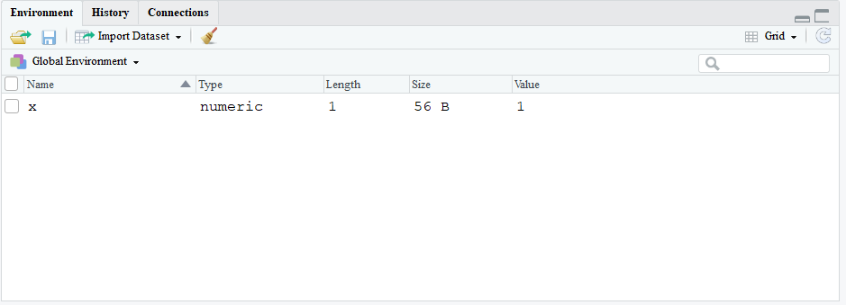
Grid style with saved object x
3.8 Putting It All Together: read.csv
Now that we understand R functions and objects, let us see how these concepts relate by again reading in a dataset using read.csv(). Again, we read in the AOSI data and save it in R as an object called excel_data.
excel_data <- read.csv("Data/cross-sec_aosi.csv")When working with a dataset, it is important to make sure all of the variables are of the correct object type (numeric, character, etc.) and that missing values are correctly labeled as NA when the dataset is read into R. This because, from before, functions operate differently based on the type of data that is being used (recall the example where we tried to take the mean of a character variable). We can view the type of each column using sapply(excel_data, class). The sapply() function is more advanced so we do not cover it here; those that are interested can view Chapter 10.
sapply(excel_data, class)## Identifiers GROUP
## "integer" "factor"
## Study_Site Gender
## "factor" "factor"
## V06.aosi.Candidate_Age V06.aosi.total_score_1_18
## "factor" "factor"
## V12.aosi.Candidate_Age V12.aosi.total_score_1_18
## "factor" "factor"We see that variables which we would think of as numeric such as AOSI total score and Age are factor variables. Let’s look at month 12 AOSI total score more closely.
excel_data$V06.aosi.total_score_1_18## [1] 8 18 4 . 6 . 16 10 . . 8 10 . 9 6 11 . . 3 18 14 . 12
## [24] 14 18 . . 5 5 5 12 11 10 7 8 12 10 8 9 11 16 9 10 18 12 11
## [47] 13 16 13 12 5 7 14 8 13 9 12 15 10 8 10 5 9 12 10 12 10 12
## [70] 12 12 11 9 12 9 9 . 15 10 10 3 . 2 9 19 10 10 11 11 8 4
## [93] 18 6 8 6 . 15 9 12 16 9 10 12 15 11 8 10 20 8 4 14 11 15 22
## [116] 16 . 9 14 12 13 22 20 10 12 12 6 14 20 12 11 7 10 . 5 .
## [139] 10 12 11 . 12 . . 14 . 9 19 12 . 6 7 9 11 . 15 10 13 10 19
## [162] 7 8 8 15 5 17 5 8 6 8 12 8 17 8 6 8 15 11 6 5 5 6 13
## [185] 9 7 5 15 4 6 9 6 4 3 14 1 4 9 9 24 12 6 5 5
## [208] . 5 15 9 10 7 10 11 8 10 13 5 12 . 6 3 3 7 12 6 17 10
## [231] . 6 11 8 . 12 5 11 16 11 7 17 16 8 12 8 10 10 11 11 12 7 5
## [254] 8 14 . 17 8 7 3 5 14 12 . 10 12 4 7 6 . 7 . 12 10 12 .
## [277] 10 15 12 12 12 2 7 7 . . . 2 11 11 . 9 15 . . . 7 9 17
## [300] 4 6 6 . 11 12 . . . 11 14 15 11 14 17 6 . 10 4 5 9 7 7
## [323] . . 18 9 . . . 17 9 . 13 11 16 7 12 17 . 11 11 12 8 3
## [346] 8 9 8 8 14 11 . 6 17 . . 28 16 11 11 7 15 . . 4 21 6 8
## [369] 10 5 9 14 13 12 7 10 . 15 7 . . 8 8 7 12 11 9 8 11 6 3
## [392] 9 8 9 4 7 8 14 6 9 15 7 9 6 11 6 6 8 9 8 7 19 15 18
## [415] 10 12 5 5 . 7 9 . . . 14 11 4 6 10 10 7 5 . 17 .
## [438] . 17 . 9 . . 13 . 11 9 . . 2 13 4 5 7 8 4 9 6
## [461] 5 . 7 . 6 11 15 8 7 5 . 4 9 6 6 6 3 6 7 7 2 5 11
## [484] 4 9 5 10 5 16 . 7 4 8 9 . 17 7 8 7 . 8 . 4 9 . 24
## [507] 13 5 7 8 6 12 5 . 3 8 9 6 6 9 7 7 6 10 11 7 14 4 .
## [530] 7 8 5 7 7 5 5 12 10 15 9 12 10 9 13 6 . 7 . . 7 . 11
## [553] 3 7 7 6 3 7 13 7 8 4 13 15 . . 8 . 3 5 8 2 6 8
## [576] 16 5 . 12 . 9 7 7 5 6 10
## 26 Levels: . 1 10 11 12 13 14 15 16 17 18 19 2 20 21 22 24 28 3 4 5 ... 9We see that the Excel sheet data for this variable has values in the form “.” and " “, which are meant to denote missing values. R considers these entries to be character values. As a result, since each column is a vector and thus each column needs to be a single type, R reads this column as a character variable. However, didn’t R tell us that this was a factor variable? This is due to the argument stringsAsFactors in read.csv(). This argument is set to TRUE by default; hence, R converts the character variable to a factor variable. This is generally what we to do with variables that are supposed to be character variables as you will see later (for example, gender). Setting it to FALSE keeps the variables as character variables. However, we do not want to consider variables like AOSI total score as character or factor variables. To do this, we need to tell R to consider the values”." and " " as missing values or NA. If this is done, then R will read the column as a collection of numbers and NA values, resulting in numeric being chosen as the variable’s type. To do this, we use the na.strings argument. By default, this argument is “NA”, implying that any values marked “NA” in the Excel sheet will be marked as missing (NA) when read in R. However, we often use different values to denote missing values (as seen here with “.” and " “). To select the values to be denoted as missing, we use **na.strings=c(“.”, " “)** in this example. That is, we provide a vector which contains the strings used to mark missing values as the value for na.strings.
excel_data <- read.csv("Data/cross-sec_aosi.csv", na.strings=c(".", " "))
excel_data$V06.aosi.total_score_1_18
## [1] 8 18 4 NA 6 NA 16 10 NA NA 8 10 NA 9 6 11 NA NA 3 18 14 NA 12
## [24] 14 18 NA NA 5 5 5 12 11 10 7 8 12 10 8 9 11 16 9 10 18 12 11
## [47] 13 16 13 12 5 NA 7 14 8 13 9 12 15 10 8 10 5 9 12 10 12 10 12
## [70] 12 12 11 9 12 NA 9 9 NA 15 10 10 3 NA 2 9 19 10 10 11 11 8 4
## [93] 18 6 8 6 NA 15 9 12 16 9 10 12 15 11 8 10 20 8 4 14 11 15 22
## [116] 16 NA NA 9 14 12 13 22 20 10 12 12 NA 6 14 20 12 11 7 10 NA 5 NA
## [139] 10 12 11 NA 12 NA NA 14 NA 9 19 12 NA 6 7 9 11 NA 15 10 13 10 19
## [162] 7 8 8 15 5 17 5 8 6 8 12 8 17 8 6 8 15 11 6 5 5 6 13
## [185] 9 7 5 15 4 6 9 6 4 3 14 1 4 9 9 24 NA 12 NA 6 NA 5 5
## [208] NA 5 15 9 10 7 10 11 8 10 13 5 12 NA 6 3 3 7 NA 12 6 17 10
## [231] NA 6 11 8 NA 12 5 11 16 11 7 17 16 8 12 8 10 10 11 11 12 7 5
## [254] 8 14 NA 17 8 7 3 5 14 12 NA 10 12 4 7 6 NA 7 NA 12 10 12 NA
## [277] 10 15 12 12 12 2 7 7 NA NA NA 2 11 11 NA 9 15 NA NA NA 7 9 17
## [300] 4 6 6 NA 11 12 NA NA NA 11 14 15 11 14 17 6 NA 10 4 5 9 7 7
## [323] NA NA 18 9 NA NA NA NA 17 9 NA 13 11 16 7 12 17 NA 11 11 12 8 3
## [346] 8 9 8 8 14 11 NA 6 17 NA NA 28 16 11 11 7 15 NA NA 4 21 6 8
## [369] 10 5 9 14 13 12 7 10 NA 15 7 NA NA 8 8 7 12 11 9 8 11 6 3
## [392] 9 8 9 4 7 8 14 6 9 15 7 9 6 11 6 6 8 9 8 7 19 15 18
## [415] 10 12 5 NA 5 NA 7 9 NA NA NA 14 11 4 6 10 10 7 NA 5 NA 17 NA
## [438] NA 17 NA 9 NA NA NA 13 NA 11 9 NA NA NA 2 13 4 5 7 8 4 9 6
## [461] 5 NA 7 NA 6 11 15 8 7 5 NA 4 9 6 6 6 3 6 7 7 2 5 11
## [484] 4 9 5 10 5 16 NA 7 4 8 9 NA 17 7 8 7 NA 8 NA 4 9 NA 24
## [507] 13 5 7 8 6 12 5 NA 3 8 9 6 6 9 7 7 6 10 11 7 14 4 NA
## [530] 7 8 5 7 7 5 5 12 10 15 9 12 10 9 13 6 NA 7 NA NA 7 NA 11
## [553] 3 7 7 6 3 7 13 7 8 4 13 15 NA NA 8 NA NA 3 5 8 2 6 8
## [576] 16 5 NA 12 NA 9 7 7 5 NA 6 10sapply(excel_data, class)## Identifiers GROUP
## "integer" "factor"
## Study_Site Gender
## "factor" "factor"
## V06.aosi.Candidate_Age V06.aosi.total_score_1_18
## "numeric" "integer"
## V12.aosi.Candidate_Age V12.aosi.total_score_1_18
## "numeric" "integer"Now, we see that missing values are marked by NA and numeric variables are correctly read-in as numeric (or integer which is a type of numeric variable) by R.