Topics

2.1 Effect Measures for Continuous Outcomes （連續反應變項的效果量）
2.2 Fixed Effect Model （固定效果模型）
2.3 Random Effects Model （隨機效果模型）
2.4 Tests and Measures of Heterogeneity （異質性的測量和檢定）
2.5 Subgroup Analysis （次群組分析）
2.6 Meta-Analysis of Other Outcomes （其他反應變項的後設分析）
2.7 Summary

Prepartion

The web-appendix here http://meta-analysis-with-r.org/.
- Datasets/
  - dataset01.csv
  - dataset02.csv
  - dataset03.csv
  - dataset04.csv
  - dataset05.csv
  - dataset06.csv
- R Code/Chapter 2: 02-continuous.R
The meta package

使用 `meta` package

!!! 安裝 meta 套件，需要花一點時間，請先執行這一行！ (後面才有辦法執行)

Code

# install.packages('meta')

Code

library(meta)

Loading 'meta' package (version 6.5-0).
Type 'help(meta)' for a brief overview.
Readers of 'Meta-Analysis with R (Use R!)' should install
older version of 'meta' package: https://tinyurl.com/dt4y5drs

Code

# Colab 環境已經預安裝 tidyverse
library(tidyverse)

── Attaching core tidyverse packages ──────────────────────── tidyverse 2.0.0 ──
✔ dplyr     1.1.4     ✔ readr     2.1.4
✔ forcats   1.0.0     ✔ stringr   1.5.1
✔ ggplot2   3.4.4     ✔ tibble    3.2.1
✔ lubridate 1.9.3     ✔ tidyr     1.3.0
✔ purrr     1.0.2

── Conflicts ────────────────────────────────────────── tidyverse_conflicts() ──
✖ dplyr::filter() masks stats::filter()
✖ dplyr::lag()    masks stats::lag()
ℹ Use the conflicted package (<http://conflicted.r-lib.org/>) to force all conflicts to become errors

Code

# 調整圖片尺寸
library(repr)
options(repr.plot.width = 12, repr.plot.height = 10)

2.1 Effect Measures for Continuous Outcomes

Code

# 資料來源網址
datasets <- 'https://www.uniklinik-freiburg.de/fileadmin/mediapool/08_institute/biometrie-statistik/Dateien/Englisch/Studies_and_Teaching/Educational_Books/Meta-Analysis_with_R/Datasets/'

Code

# 1. Read in the data
data1 <- read.csv(paste0(datasets, 'dataset01.csv'))
data1

         author  year Ne    Me    Se Nc    Mc    Sc
1         Boner  1988 13 13.54 13.85 13 20.77 21.46
2         Boner  1989 20 15.70 13.10 20 22.70 16.47
3        Chudry  1987 12 21.30 13.10 12 39.70 12.90
4         Comis  1993 12 14.50 12.20 12 31.30 15.10
5  DeBenedictis 1994a 17 14.40 11.10 17 27.40 17.30
6  DeBenedictis 1994b  8 14.80 18.60  8 31.40 20.60
7  DeBenedictis  1995 13 15.70 16.80 13 29.60 18.90
8       Debelic  1986 12 29.83 15.95 12 48.08 15.08
9     Henriksen  1988 12 17.50 13.10 12 47.20 16.47
10        Konig  1987 12 12.00 14.60 12 26.20 12.30
11       Morton  1992 16 15.83 13.43 16 38.36 18.01
12     Novembre 1994f 24 15.42  8.35 24 28.46 13.84
13     Novembre 1994s 19 11.00 12.40 19 26.10 14.90
14        Oseid  1995 20 14.10  9.50 20 28.90 18.00
15      Roberts  1985  9 18.90 17.70  9 38.90 18.90
16         Shaw  1985  8 10.27  7.02  8 34.43 10.96
17       Todaro  1993 13 10.10  8.90 13 23.50  4.00

2.1.1 Mean Difference 課本寫法

The estimated mean difference. \(\hat \mu_k = \hat \mu_{ek} - \hat \mu_{ck}\)
The variance estimate. \(\hat{Var}(\hat \mu_k) = \dfrac{s_{ek}^2}{n_{ek}} + \dfrac{s_{ck}^2}{n_{ck}}\)
An approximate two-sided (\(1-\alpha\)) confidence interval. \((\hat \mu_{ek} - \hat \mu_{ck}) \pm z_{1-\frac{\alpha}{2}} \sqrt{\dfrac{s_{ek}^2}{n_{ek}} + \dfrac{s_{ck}^2}{n_{ck}}}\)

Example 2.1 (p.23)

Code

# 2. Calculate mean difference and its standard error for
#    study 1 (Boner 1988) of dataset data1:
MD <- with(data1[1, ], Me - Mc)
seMD <- with(data1[1, ], sqrt(Se^2 / Ne + Sc^2 / Nc))
# 3. Print mean difference and limits of 95% confidence
#    interval using round function to show only two digits:
round(c(MD, MD + c(-1, 1) * qnorm(1 - (0.05 / 2)) * seMD), 2)

[1]  -7.23 -21.11   6.65

Code

zscore <- MD / seMD
round(c(zscore, 2 * pnorm(abs(zscore), lower.tail = FALSE)), 4)

[1] -1.0206  0.3074

`metacont` 的結果

兩種寫法是一樣的

Code

# method 1
with(data1[1, ],
     print(metacont(Ne, Me, Se, Nc, Mc, Sc),
           digits=2))

Number of observations: o = 26

    MD         95%-CI     z p-value
 -7.23 [-21.11; 6.65] -1.02  0.3074

Code

# method 2
print(metacont(Ne, Me, Se, Nc, Mc, Sc,
               data=data1, subset=1), digits=2)

Number of observations: o = 26

     MD         95%-CI     z p-value
1 -7.23 [-21.11; 6.65] -1.02  0.3074

(2.1.1 Note.) Tidy-style 寫法

Code

# data1 <- read_csv("dataset01.csv")
data1 |>
  slice(1) |>
  summarise(
    md = Me - Mc,
    se_md = sqrt(Se^2 / Ne + Sc^2 / Nc),
    ci_lower = md - qnorm(1 - (0.05 / 2)) * se_md,
    ci_upper = md + qnorm(1 - (0.05 / 2)) * se_md,
    z_score = md/se_md,
    p_value = 2*pnorm(abs(z_score), lower.tail=FALSE)  # Pr(X > x)
  )

     md    se_md  ci_lower ci_upper  z_score   p_value
1 -7.23 7.083861 -21.11411 6.654112 -1.02063 0.3074298

Code

data1 |>
  slice(1) |>
  metacont(
    data = _,
    n.e = Ne, 
    mean.e = Me, 
    sd.e = Se, 
    n.c = Nc, 
    mean.c = Mc, 
    sd.c = Sc,
    sm = "MD" # default
  )

Number of observations: o = 26

      MD             95%-CI     z p-value
 -7.2300 [-21.1141; 6.6541] -1.02  0.3074

2.1.2 Standardised Mean Difference 課本寫法

The standardised mean difference (SMD) which is called Hedges’s g. \(\hat g_k = \left(1-\dfrac{3}{4n_k - 9}\right)\dfrac{\hat \mu_{ek} - \hat \mu_{ck}}{\sqrt{\dfrac{(n_{ek}-1)s_{ek}^2 + (n_{ck}-1)s_{ck}^2}{n_k-2}}}\)
Variance. \(\hat Var(\hat g_k) = \dfrac{n_k}{n_{ek} \cdot n_{ck}} + \dfrac{\hat g_k^2}{2(n_k - 3.94)}\)
1. \(\hat g_k \pm z_{1-\frac{1}{2}}SE(\hat g_k)\)

Example 2.2 (p.26)

Code

data2 <- read.csv(paste0(datasets, "dataset02.csv"))
# 2. As usual, to view an object, type its name:
data2

              author  Ne    Me    Se Nc    Mc    Sc
1    Blashki(75%150)  13  6.40  5.40 18 11.40  9.60
2     Hormazabal(86)  17 11.00  8.20 16 19.00  8.20
3   Jacobson(75-100)  10 17.50  8.80  6 23.00  8.80
4        Jenkins(75)   7 12.30  9.90  7 20.00 10.50
5     Lecrubier(100)  73 15.70 10.60 73 18.70 10.60
6        Murphy(100)  26  8.50 11.00 28 14.50 11.00
7          Nandi(97)  17 25.50 24.00 10 53.20 11.20
8      Petracca(100)  11  6.20  7.60 10 10.00  7.60
9       Philipp(100) 105 -8.10  3.90 46 -8.50  5.20
10     Rampello(100)  22 13.40  2.30 19 19.70  1.30
11       Reifler(83)  13 12.50  7.60 15 12.50  7.60
12       Rickels(70)  29  1.99  0.77 39  2.54  0.77
13     Robertson(75)  13 11.00  8.20 13 15.00  8.20
14      Rouillon(98)  78 15.80  6.80 71 17.10  7.20
15           Tan(70)  23 -8.50  8.60 23 -8.30  6.00
16 Tetreault(50-100)  11 51.90 18.50 11 74.30 18.50
17      Thompson(75)  11  8.00  8.10 18 10.00  9.70

Code

# 3. Calculate total sample sizes
summary(data2$Ne + data2$Nc)

   Min. 1st Qu.  Median    Mean 3rd Qu.    Max. 
  14.00   26.00   31.00   53.06   54.00  151.00

Code

# 1. Calculate standardised mean difference (SMD) and
#    its standard error (seSMD) for study 1 (Blashki) of
#    dataset data2:
N <- with(data2[1, ], Ne + Nc)
SMD <- with(
  data2[1, ],
  (1 - 3 / (4 * N - 9)) * (Me - Mc) /
    sqrt(((Ne - 1) * Se^2 + (Nc - 1) * Sc^2) / (N - 2))
)
seSMD <- with(
  data2[1, ],
  sqrt(N / (Ne * Nc) + SMD^2 / (2 * (N - 3.94)))
)
# 2. Print standardised mean difference and limits of 95% CI
#    interval using round function to show only two digits:
round(c(SMD, SMD + c(-1, 1) * qnorm(1 - (0.05 / 2)) * seSMD), 2)

[1] -0.60 -1.33  0.13

Code

metacont(
  Ne, Me, Se, Nc, Mc, Sc,
  sm = "SMD",
  data = data2, 
  subset = 1
)

Number of observations: o = 31

      SMD            95%-CI     z p-value
1 -0.5990 [-1.3299; 0.1319] -1.61  0.1082

Details:
- Hedges' g (bias corrected standardised mean difference; using exact formulae)

(2.1.2 Note.) Tidy-style 寫法

Code

data2 |>
  slice(1) |>
  summarise(
  n = Ne + Nc,
  smd =   (1 - 3 / (4 * N - 9)) * (Me - Mc) /
    sqrt(((Ne - 1) * Se^2 + (Nc - 1) * Sc^2) / (N - 2)),
  se_smd = sqrt(N / (Ne * Nc) + SMD^2 / (2 * (N - 3.94))),
  ci_lower = smd - qnorm(1 - (0.05 / 2)) * se_smd,
  ci_upper = smd + qnorm(1 - (0.05 / 2)) * se_smd,
  z_score = smd/se_smd,
  p_value = 2*pnorm(abs(z_score), lower.tail=FALSE)
  )

   n        smd   se_smd  ci_lower  ci_upper   z_score   p_value
1 31 -0.5989891 0.372972 -1.330001 0.1320226 -1.605989 0.1082762

Code

data2 |>
  slice(1) |>
  metacont(
    data = _,
    n.e = Ne, 
    mean.e = Me, 
    sd.e = Se, 
    n.c = Nc, 
    mean.c = Mc, 
    sd.c = Sc,
    sm = "SMD"
  )

Number of observations: o = 31

     SMD            95%-CI     z p-value
 -0.5990 [-1.3299; 0.1319] -1.61  0.1082

Details:
- Hedges' g (bias corrected standardised mean difference; using exact formulae)

2.2 Fixed Effect Model

The fixed effect model is

\[\hat \theta_k = \theta + \sigma_k \epsilon_k,\\ \epsilon_k \overset{\mathrm{iid}}{\sim} N(0,1) \]

Estimate. \(\hat \theta_F = \dfrac{\sum \limits_{k=1}^K \hat \theta_k / \hat \sigma_k ^2}{\sum \limits_{k=1}^K 1 / \hat \sigma_k ^2} = \dfrac{\sum \limits_{k=1}^K w_k \hat \theta_k}{\sum \limits_{k=1}^K w_k}\)
Variance. \(\hat Var(\hat \theta_F) = \dfrac{1}{\sum \limits_{k=1}^K w_k}\)
1. \(\hat \theta_F \pm z_{1-\frac{\alpha}{2}} SE(\hat \theta_F)\)
The inverse variance method. \(w_k = \dfrac{1}{\hat \sigma_k^2}\)

The fixed effect estimate \(\hat \theta_F\) and its variance can be calculated using the following quantities:

(考慮一開始的 fixed effect model)

\(\hat \theta_k = \hat \mu_k\)
\(\hat \sigma_k^2 = \hat Var(\hat \mu_k)\)

Or in SMD,

\(\hat \theta_k = \hat g_k\)
\(\hat \sigma_k^2 = \hat Var(\hat g_k)\)

Example 2.3 (p.29)

Code

# 1. Calculate mean difference, variance and weights
MD <- with(data1, Me - Mc)
varMD <- with(data1, Se^2 / Ne + Sc^2 / Nc)
weight <- 1 / varMD
# 2. Calculate the inverse variance estimator
round(weighted.mean(MD, weight), 4)

[1] -15.514

Code

# 3. Calculate the variance
round(1 / sum(weight), 4)

[1] 1.4126

Code

mc1 <- metacont(Ne, Me, Se, Nc, Mc, Sc,
  data = data1,
  studlab = paste(author, year),
  # method.tau = "DL" 要設定才會跟課本一樣！ 
  method.tau = "DL"
)

# 跟上一格比較
round(c(mc1$TE.fixed, mc1$seTE.fixed^2), 4)

[1] -15.5140   1.4126

Code

summary(mc1)

                         MD               95%-CI %W(common) %W(random)
Boner 1988          -7.2300 [-21.1141;   6.6541]        2.8        3.1
Boner 1989          -7.0000 [-16.2230;   2.2230]        6.4        6.6
Chudry 1987        -18.4000 [-28.8023;  -7.9977]        5.0        5.3
Comis 1993         -16.8000 [-27.7835;  -5.8165]        4.5        4.8
DeBenedictis 1994a -13.0000 [-22.7710;  -3.2290]        5.7        5.9
DeBenedictis 1994b -16.6000 [-35.8326;   2.6326]        1.5        1.6
DeBenedictis 1995  -13.9000 [-27.6461;  -0.1539]        2.9        3.1
Debelic 1986       -18.2500 [-30.6692;  -5.8308]        3.5        3.8
Henriksen 1988     -29.7000 [-41.6068; -17.7932]        3.8        4.1
Konig 1987         -14.2000 [-25.0013;  -3.3987]        4.7        4.9
Morton 1992        -22.5300 [-33.5382; -11.5218]        4.5        4.8
Novembre 1994f     -13.0400 [-19.5067;  -6.5733]       13.0       12.1
Novembre 1994s     -15.1000 [-23.8163;  -6.3837]        7.1        7.3
Oseid 1995         -14.8000 [-23.7200;  -5.8800]        6.8        7.0
Roberts 1985       -20.0000 [-36.9171;  -3.0829]        1.9        2.1
Shaw 1985          -24.1600 [-33.1791; -15.1409]        6.7        6.9
Todaro 1993        -13.4000 [-18.7042;  -8.0958]       19.3       16.6

Number of studies: k = 17
Number of observations: o = 480

                           MD               95%-CI      z  p-value
Common effect model  -15.5140 [-17.8435; -13.1845] -13.05 < 0.0001
Random effects model -15.6436 [-18.1369; -13.1502] -12.30 < 0.0001

Quantifying heterogeneity:
 tau^2 = 2.4374 [0.0000; 40.8996]; tau = 1.5612 [0.0000; 6.3953]
 I^2 = 8.9% [0.0%; 45.3%]; H = 1.05 [1.00; 1.35]

Test of heterogeneity:
     Q d.f. p-value
 17.57   16  0.3496

Details on meta-analytical method:
- Inverse variance method
- DerSimonian-Laird estimator for tau^2
- Jackson method for confidence interval of tau^2 and tau

Code

mc1$w.fixed[1]

[1] 0.01992783

Code

sum(mc1$w.fixed)

[1] 0.7079028

Code

round(100 * mc1$w.fixed[1] / sum(mc1$w.fixed), 2)

[1] 2.82

Code

# pdf(file="Schwarzer-Fig2.3.pdf", width=9.6) # uncomment line to generate PDF file
forest(mc1,
  comb.random = FALSE, xlab =
    "Difference in mean response (intervention - control)
units: maximum % fall in FEV1",
  xlim = c(-50, 10), xlab.pos = -20, smlab.pos = -20
)

Code

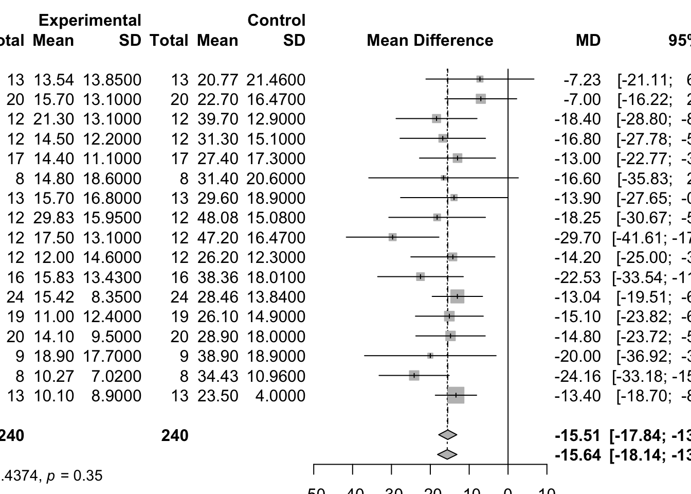
# invisible(dev.off()) # uncomment line to save PDF file

Code

# 1. Apply generic inverse variance method
mc1.gen <- metagen(mc1$TE, mc1$seTE, sm = "MD")
# 2. Same result
mc1.gen <- metagen(TE, seTE, data = mc1, sm = "MD")
# 3. Print results for fixed effect and random effects method
c(mc1$TE.fixed, mc1$TE.random)

[1] -15.51403 -15.64357

Code

c(mc1.gen$TE.fixed, mc1.gen$TE.random)

[1] -15.51403 -15.64702

Example 2.4 (p.33)

Code

# 1. Calculate standardised mean difference,
#    variance and weights
N <- with(data2, Ne + Nc)
SMD <- with(
  data2,
  (1 - 3 / (4 * N - 9)) * (Me - Mc) /
    sqrt(((Ne - 1) * Se^2 + (Nc - 1) * Sc^2) / (N - 2))
)
varSMD <- with(
  data2,
  N / (Ne * Nc) + SMD^2 / (2 * (N - 3.94))
)
weight <- 1 / varSMD
# 2. Calculate the inverse variance estimator
round(weighted.mean(SMD, weight), 4)

[1] -0.3915

Code

# 3. Calculate the variance
round(1 / sum(weight), 4)

[1] 0.0049

Code

mc2 <- metacont(
  Ne, Me, Se, Nc, Mc, Sc,
  sm = "SMD",
  data = data2,
  # method.tau = "DL" 要設定才會跟課本一樣！ 
  method.tau = "DL"
)
round(c(mc2$TE.fixed, mc2$seTE.fixed^2), 4)

[1] -0.3918  0.0049

Code

summary(mc2)

       SMD             95%-CI %W(common) %W(random)
1  -0.5990 [-1.3299;  0.1319]        3.5        5.7
2  -0.9518 [-1.6767; -0.2268]        3.6        5.7
3  -0.5908 [-1.6296;  0.4480]        1.7        4.1
4  -0.7062 [-1.7975;  0.3850]        1.6        3.9
5  -0.2815 [-0.6076;  0.0445]       17.6        8.1
6  -0.5375 [-1.0816;  0.0065]        6.3        6.8
7  -1.3204 [-2.1888; -0.4520]        2.5        4.9
8  -0.4800 [-1.3512;  0.3913]        2.5        4.9
9   0.0918 [-0.2549;  0.4385]       15.6        8.0
10 -3.2433 [-4.2020; -2.2846]        2.0        4.5
11  0.0000 [-0.7427;  0.7427]        3.4        5.6
12 -0.7061 [-1.2020; -0.2103]        7.6        7.1
13 -0.4724 [-1.2536;  0.3088]        3.1        5.4
14 -0.1849 [-0.5071;  0.1372]       18.0        8.2
15 -0.0265 [-0.6045;  0.5515]        5.6        6.6
16 -1.1647 [-2.0819; -0.2476]        2.2        4.7
17 -0.2127 [-0.9651;  0.5397]        3.3        5.6

Number of studies: k = 17
Number of observations: o = 902

                         SMD             95%-CI     z  p-value
Common effect model  -0.3918 [-0.5286; -0.2551] -5.62 < 0.0001
Random effects model -0.5861 [-0.8709; -0.3014] -4.03 < 0.0001

Quantifying heterogeneity:
 tau^2 = 0.2315 [0.1379; 0.9822]; tau = 0.4812 [0.3714; 0.9911]
 I^2 = 72.6% [55.5%; 83.1%]; H = 1.91 [1.50; 2.43]

Test of heterogeneity:
     Q d.f.  p-value
 58.38   16 < 0.0001

Details on meta-analytical method:
- Inverse variance method
- DerSimonian-Laird estimator for tau^2
- Jackson method for confidence interval of tau^2 and tau
- Hedges' g (bias corrected standardised mean difference; using exact formulae)

2.3 Random Effects Model

The random effect model is

\[\hat \theta_k = \theta + \mu_k + \sigma_k \epsilon_k,\\ \epsilon_k \overset{\mathrm{iid}}{\sim} N(0,1), \\ u_k \overset{\mathrm{iid}}{\sim} N(0,\tau^2)\]

Q statistcis. \(Q = \sum \limits_{k=1}^K w_k (\hat \theta_k - \hat \theta_F)^2,\\ w_k=1/\hat \sigma^2\)
between-study variance. \(\hat \tau^2 = \dfrac{Q - (K-1)}{S}\)

ANd the random effects estimate and its variance are given by

Estimate. \(\hat \theta_R = \dfrac{\sum \limits_{k=1}^K w_k^* \hat \theta_k}{\sum \limits_{k=1}^K w_k^*}\)
Variance. \(\hat Var(\hat \theta_R) = \dfrac{1}{\sum \limits_{k=1}^K w_k^*}\)
1. \(\hat \theta_R \pm z_{1-\frac{\alpha}{2}} SE(\hat \theta_R)\)
\(w_k^* = \dfrac{1}{\hat \sigma_k^2 + \hat \tau^2}\)

2.3.1 Estimation of Between-Study Variance

The following methods to estimate the between-study variance \(\tau^2\) are available in the metagen and other functions of R package meta (argument method.tau):

DerSimonian–Laird estimator (method.tau="DL") (課本 2014 年當時 default)
Paule–Mandel estimator (method.tau="PM")
Restricted maximum-likelihood estimator (method.tau="REML") (現在 meta 6.2-1 default)
Maximum-likelihood estimator (method.tau="ML")
Hunter–Schmidt estimator (method.tau="HS")
Sidik–Jonkman estimator (method.tau="SJ")
Hedges estimator (method.tau="HE")
Empirical Bayes estimator (method.tau="EB")

2.3.2 Hartung–Knapp Adjustment

Variance.(參見 Q 統計量。) \(\hat{Var}_{HK} (\hat \theta_R) = \dfrac{1}{K-1} \sum \limits_{k=1}^K \dfrac{w_k^*}{w^*} (\hat \theta_k - \hat \theta_R)^2,\\ w_k^*=1/ (\hat \sigma^2 + \hat \tau^2),\\ w^* = \sum_{k=1}^K w_k^*\)
1. \(\hat \theta_R \pm t_{(K-1, 1-\frac{\alpha}{2})} SE_{HK}(\hat \theta_R)\)

Example 2.8 (p.38)

Code

mc2.hk1 <- metacont(
  Ne, Me, Se, Nc, Mc, Sc,
  sm = "SMD",
  data = data2, comb.fixed = FALSE,
  # method.tau = "DL" 要設定才會跟課本一樣！ 
  method.tau = "DL",
  method.random.ci = "HK", # hakn = TRUE,
  method.tau.ci = ""
)

summary(mc2.hk1)

       SMD             95%-CI %W(random)
1  -0.5990 [-1.3299;  0.1319]        5.7
2  -0.9518 [-1.6767; -0.2268]        5.7
3  -0.5908 [-1.6296;  0.4480]        4.1
4  -0.7062 [-1.7975;  0.3850]        3.9
5  -0.2815 [-0.6076;  0.0445]        8.1
6  -0.5375 [-1.0816;  0.0065]        6.8
7  -1.3204 [-2.1888; -0.4520]        4.9
8  -0.4800 [-1.3512;  0.3913]        4.9
9   0.0918 [-0.2549;  0.4385]        8.0
10 -3.2433 [-4.2020; -2.2846]        4.5
11  0.0000 [-0.7427;  0.7427]        5.6
12 -0.7061 [-1.2020; -0.2103]        7.1
13 -0.4724 [-1.2536;  0.3088]        5.4
14 -0.1849 [-0.5071;  0.1372]        8.2
15 -0.0265 [-0.6045;  0.5515]        6.6
16 -1.1647 [-2.0819; -0.2476]        4.7
17 -0.2127 [-0.9651;  0.5397]        5.6

Number of studies: k = 17
Number of observations: o = 902

                         SMD             95%-CI     t p-value
Random effects model -0.5861 [-0.9514; -0.2209] -3.40  0.0036

Quantifying heterogeneity:
 tau^2 = 0.2315; tau = 0.4812; I^2 = 72.6% [55.5%; 83.1%]; H = 1.91 [1.50; 2.43]

Test of heterogeneity:
     Q d.f.  p-value
 58.38   16 < 0.0001

Details on meta-analytical method:
- Inverse variance method
- DerSimonian-Laird estimator for tau^2
- Hartung-Knapp adjustment for random effects model (df = 16)
- Hedges' g (bias corrected standardised mean difference; using exact formulae)

Code

mc2.hk <- metagen(
  TE, seTE,
  data = mc2, comb.fixed = FALSE,
  # method.tau = "DL" 要設定才會跟課本一樣！ 
  method.tau = "DL",
  method.random.ci = "HK", # hakn = TRUE,
  method.tau.ci = ""
)

summary(mc2.hk)

                       95%-CI %W(random)
1  -0.5990 [-1.3299;  0.1319]        5.7
2  -0.9518 [-1.6767; -0.2268]        5.7
3  -0.5908 [-1.6296;  0.4480]        4.1
4  -0.7062 [-1.7975;  0.3850]        3.9
5  -0.2815 [-0.6076;  0.0445]        8.1
6  -0.5375 [-1.0816;  0.0065]        6.8
7  -1.3204 [-2.1888; -0.4520]        4.9
8  -0.4800 [-1.3512;  0.3913]        4.9
9   0.0918 [-0.2549;  0.4385]        8.0
10 -3.2433 [-4.2020; -2.2846]        4.5
11  0.0000 [-0.7427;  0.7427]        5.6
12 -0.7061 [-1.2020; -0.2103]        7.1
13 -0.4724 [-1.2536;  0.3088]        5.4
14 -0.1849 [-0.5071;  0.1372]        8.2
15 -0.0265 [-0.6045;  0.5515]        6.6
16 -1.1647 [-2.0819; -0.2476]        4.7
17 -0.2127 [-0.9651;  0.5397]        5.6

Number of studies: k = 17

                                              95%-CI     t p-value
Random effects model (HK) -0.5861 [-0.9514; -0.2209] -3.40  0.0036

Quantifying heterogeneity:
 tau^2 = 0.2315; tau = 0.4812; I^2 = 72.6% [55.5%; 83.1%]; H = 1.91 [1.50; 2.43]

Test of heterogeneity:
     Q d.f.  p-value
 58.38   16 < 0.0001

Details on meta-analytical method:
- Inverse variance method
- DerSimonian-Laird estimator for tau^2
- Hartung-Knapp adjustment for random effects model (df = 16)

2.3.3 Prediction Intervals 課本寫法

1. \(\hat \theta_R \pm t_{(K-2, 1-\frac{\alpha}{2})} \sqrt{\hat{Var}(\hat \theta_R)+\hat \tau^2}\)

Example 2.9 (p.39)

Code

# 現在要把 prediction = TRUE 設定在 metacont() function
mc1_pred <- metacont(Ne, Me, Se, Nc, Mc, Sc,
  data = data1,
  studlab = paste(author, year),
  # method.tau = "DL" 要設定才會跟課本一樣！ 
  method.tau = "DL",
  prediction = TRUE
)

summary(mc1_pred)

                         MD               95%-CI %W(common) %W(random)
Boner 1988          -7.2300 [-21.1141;   6.6541]        2.8        3.1
Boner 1989          -7.0000 [-16.2230;   2.2230]        6.4        6.6
Chudry 1987        -18.4000 [-28.8023;  -7.9977]        5.0        5.3
Comis 1993         -16.8000 [-27.7835;  -5.8165]        4.5        4.8
DeBenedictis 1994a -13.0000 [-22.7710;  -3.2290]        5.7        5.9
DeBenedictis 1994b -16.6000 [-35.8326;   2.6326]        1.5        1.6
DeBenedictis 1995  -13.9000 [-27.6461;  -0.1539]        2.9        3.1
Debelic 1986       -18.2500 [-30.6692;  -5.8308]        3.5        3.8
Henriksen 1988     -29.7000 [-41.6068; -17.7932]        3.8        4.1
Konig 1987         -14.2000 [-25.0013;  -3.3987]        4.7        4.9
Morton 1992        -22.5300 [-33.5382; -11.5218]        4.5        4.8
Novembre 1994f     -13.0400 [-19.5067;  -6.5733]       13.0       12.1
Novembre 1994s     -15.1000 [-23.8163;  -6.3837]        7.1        7.3
Oseid 1995         -14.8000 [-23.7200;  -5.8800]        6.8        7.0
Roberts 1985       -20.0000 [-36.9171;  -3.0829]        1.9        2.1
Shaw 1985          -24.1600 [-33.1791; -15.1409]        6.7        6.9
Todaro 1993        -13.4000 [-18.7042;  -8.0958]       19.3       16.6

Number of studies: k = 17
Number of observations: o = 480

                           MD               95%-CI      z  p-value
Common effect model  -15.5140 [-17.8435; -13.1845] -13.05 < 0.0001
Random effects model -15.6436 [-18.1369; -13.1502] -12.30 < 0.0001
Prediction interval           [-19.9360; -11.3511]                

Quantifying heterogeneity:
 tau^2 = 2.4374 [0.0000; 40.8996]; tau = 1.5612 [0.0000; 6.3953]
 I^2 = 8.9% [0.0%; 45.3%]; H = 1.05 [1.00; 1.35]

Test of heterogeneity:
     Q d.f. p-value
 17.57   16  0.3496

Details on meta-analytical method:
- Inverse variance method
- DerSimonian-Laird estimator for tau^2
- Jackson method for confidence interval of tau^2 and tau
- Prediction interval based on t-distribution (df = 15)

Code

# summary(mc1, prediction = TRUE)

Code

forest(mc1_pred, prediction = TRUE, col.predict = "black")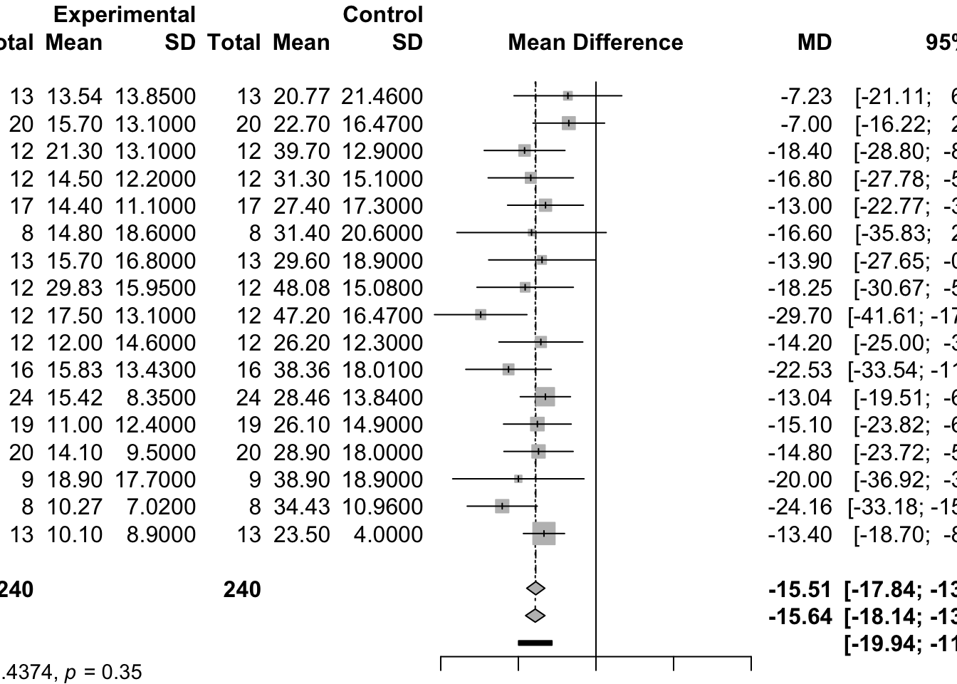

2.5 Subgroup Analysis

Example 2.12 (p.41)

Code

# 1. Read in the data:
data3 <- read.csv(paste0(datasets, "dataset03.csv"))
# 2. As usual, to view an object, type its name:
data3

        author year  Ne   Me   Se  Nc   Mc   Sc    duration
1   Bontognali 1991  30 0.70 3.76  30 1.27 4.58 <= 3 months
2  Castiglioni 1986 311 0.10 0.21 302 0.20 0.29 <= 3 months
3    Cremonini 1986  21 0.25 0.23  20 0.71 0.29 <= 3 months
4       Grassi 1994  42 0.16 0.29  41 0.45 0.43 <= 3 months
5      Jackson 1984  61 0.11 0.00  60 0.13 0.00 <= 3 months
6      Allegra 1996 223 0.07 0.11 218 0.11 0.14  > 3 months
7     Babolini 1980 254 0.13 0.18 241 0.33 0.27  > 3 months
8        Boman 1983  98 0.20 0.27 105 0.32 0.30  > 3 months
9       Borgia 1981  10 0.05 0.08   9 0.15 0.17  > 3 months
10    Decramer 2005 256 0.10 0.11 267 0.11 0.16  > 3 months
11      Grassi 1976  35 0.14 0.15  34 0.27 0.21  > 3 months
12    Grillage 1985  54 0.10 0.00  55 0.12 0.00  > 3 months
13      Hansen 1994  59 0.11 0.15  70 0.16 0.19  > 3 months
14     Malerba 2004 115 0.06 0.08 119 0.07 0.08  > 3 months
15     McGavin 1985  72 0.42 0.34  76 0.52 0.35  > 3 months
16     Meister 1986  90 0.15 0.15  91 0.20 0.19  > 3 months
17     Meister 1999 122 0.06 0.15 124 0.10 0.15  > 3 months
18     Moretti 2004  63 0.12 0.14  61 0.17 0.17  > 3 months
19       Nowak 1999 147 0.03 0.06 148 0.06 0.12  > 3 months
20    Olivieri 1987 110 0.18 0.31 104 0.33 0.41  > 3 months
21        Parr 1987 243 0.18 0.21 210 0.21 0.21  > 3 months
22        Pela 1999  83 0.17 0.18  80 0.29 0.32  > 3 months
23   Rasmussen 1988  44 0.13 0.21  47 0.14 0.19  > 3 months

Code

mc3 <- metacont(
  Ne, Me, Se, Nc, Mc, Sc,
  data = data3,
  studlab = paste(author, year),
  # method.tau = "DL" 要設定才會跟課本一樣！ 
  method.tau = "DL"
)

Warning in metacont(Ne, Me, Se, Nc, Mc, Sc, data = data3, studlab =
paste(author, : Note, studies with non-positive values for sd.e or sd.c get no
weight in meta-analysis.

Code

mc3$studlab[mc3$w.fixed == 0]

[1] "Jackson 1984"  "Grillage 1985"

Code

summary(mc3)

                      MD             95%-CI %W(common) %W(random)
Bontognali 1991  -0.5700 [-2.6904;  1.5504]        0.0        0.0
Castiglioni 1986 -0.1000 [-0.1402; -0.0598]        4.9        6.2
Cremonini 1986   -0.4600 [-0.6207; -0.2993]        0.3        2.1
Grassi 1994      -0.2900 [-0.4482; -0.1318]        0.3        2.1
Jackson 1984     -0.0200                           0.0        0.0
Allegra 1996     -0.0400 [-0.0635; -0.0165]       14.2        6.7
Babolini 1980    -0.2000 [-0.2406; -0.1594]        4.8        6.1
Boman 1983       -0.1200 [-0.1984; -0.0416]        1.3        4.5
Borgia 1981      -0.1000 [-0.2216;  0.0216]        0.5        3.0
Decramer 2005    -0.0100 [-0.0334;  0.0134]       14.3        6.7
Grassi 1976      -0.1300 [-0.2163; -0.0437]        1.1        4.2
Grillage 1985    -0.0200                           0.0        0.0
Hansen 1994      -0.0500 [-0.1087;  0.0087]        2.3        5.4
Malerba 2004     -0.0100 [-0.0305;  0.0105]       18.7        6.8
McGavin 1985     -0.1000 [-0.2112;  0.0112]        0.6        3.3
Meister 1986     -0.0500 [-0.0998; -0.0002]        3.2        5.7
Meister 1999     -0.0400 [-0.0775; -0.0025]        5.6        6.3
Moretti 2004     -0.0500 [-0.1049;  0.0049]        2.6        5.5
Nowak 1999       -0.0300 [-0.0516; -0.0084]       16.8        6.8
Olivieri 1987    -0.1500 [-0.2478; -0.0522]        0.8        3.7
Parr 1987        -0.0300 [-0.0688;  0.0088]        5.2        6.2
Pela 1999        -0.1200 [-0.2001; -0.0399]        1.2        4.4
Rasmussen 1988   -0.0100 [-0.0925;  0.0725]        1.2        4.3

Number of studies: k = 21
Number of observations: o = 5055

                          MD             95%-CI      z  p-value
Common effect model  -0.0455 [-0.0544; -0.0367] -10.06 < 0.0001
Random effects model -0.0812 [-0.1085; -0.0538]  -5.82 < 0.0001

Quantifying heterogeneity:
 tau^2 = 0.0027 [0.0000; 0.0123]; tau = 0.0524 [0.0000; 0.1111]
 I^2 = 85.5% [79.1%; 89.9%]; H = 2.63 [2.19; 3.15]

Test of heterogeneity:
      Q d.f.  p-value
 138.08   20 < 0.0001

Details on meta-analytical method:
- Inverse variance method
- DerSimonian-Laird estimator for tau^2
- Jackson method for confidence interval of tau^2 and tau

Code

mc3s <- metacont(
  Ne, Me, Se, Nc, Mc, Sc,
  data = data3,
  studlab = paste(author, year),
  byvar = duration, print.byvar = FALSE,
  # method.tau = "DL" 要設定才會跟課本一樣！ 
  method.tau = "DL"
)

Warning in metacont(Ne, Me, Se, Nc, Mc, Sc, data = data3, studlab =
paste(author, : Note, studies with non-positive values for sd.e or sd.c get no
weight in meta-analysis.

Warning in metacont(x$n.e[sel], x$mean.e[sel], x$sd.e[sel], x$n.c[sel], : Note,
studies with non-positive values for sd.e or sd.c get no weight in
meta-analysis.

Warning in metacont(x$n.e[sel], x$mean.e[sel], x$sd.e[sel], x$n.c[sel], : Note,
studies with non-positive values for sd.e or sd.c get no weight in
meta-analysis.

Code

# Another way: update.meta()
mc3s <- update(
  mc3, byvar = duration, print.byvar = FALSE, 
  # method.tau = "DL" 要設定才會跟課本一樣！ 
  method.tau = "DL"
)

Code

summary(mc3s)

                      MD             95%-CI %W(common) %W(random)    duration
Bontognali 1991  -0.5700 [-2.6904;  1.5504]        0.0        0.0 <= 3 months
Castiglioni 1986 -0.1000 [-0.1402; -0.0598]        4.9        6.2 <= 3 months
Cremonini 1986   -0.4600 [-0.6207; -0.2993]        0.3        2.1 <= 3 months
Grassi 1994      -0.2900 [-0.4482; -0.1318]        0.3        2.1 <= 3 months
Jackson 1984     -0.0200                           0.0        0.0 <= 3 months
Allegra 1996     -0.0400 [-0.0635; -0.0165]       14.2        6.7  > 3 months
Babolini 1980    -0.2000 [-0.2406; -0.1594]        4.8        6.1  > 3 months
Boman 1983       -0.1200 [-0.1984; -0.0416]        1.3        4.5  > 3 months
Borgia 1981      -0.1000 [-0.2216;  0.0216]        0.5        3.0  > 3 months
Decramer 2005    -0.0100 [-0.0334;  0.0134]       14.3        6.7  > 3 months
Grassi 1976      -0.1300 [-0.2163; -0.0437]        1.1        4.2  > 3 months
Grillage 1985    -0.0200                           0.0        0.0  > 3 months
Hansen 1994      -0.0500 [-0.1087;  0.0087]        2.3        5.4  > 3 months
Malerba 2004     -0.0100 [-0.0305;  0.0105]       18.7        6.8  > 3 months
McGavin 1985     -0.1000 [-0.2112;  0.0112]        0.6        3.3  > 3 months
Meister 1986     -0.0500 [-0.0998; -0.0002]        3.2        5.7  > 3 months
Meister 1999     -0.0400 [-0.0775; -0.0025]        5.6        6.3  > 3 months
Moretti 2004     -0.0500 [-0.1049;  0.0049]        2.6        5.5  > 3 months
Nowak 1999       -0.0300 [-0.0516; -0.0084]       16.8        6.8  > 3 months
Olivieri 1987    -0.1500 [-0.2478; -0.0522]        0.8        3.7  > 3 months
Parr 1987        -0.0300 [-0.0688;  0.0088]        5.2        6.2  > 3 months
Pela 1999        -0.1200 [-0.2001; -0.0399]        1.2        4.4  > 3 months
Rasmussen 1988   -0.0100 [-0.0925;  0.0725]        1.2        4.3  > 3 months

Number of studies: k = 21
Number of observations: o = 5055

                          MD             95%-CI      z  p-value
Common effect model  -0.0455 [-0.0544; -0.0367] -10.06 < 0.0001
Random effects model -0.0812 [-0.1085; -0.0538]  -5.82 < 0.0001

Quantifying heterogeneity:
 tau^2 = 0.0027 [0.0000; 0.0123]; tau = 0.0524 [0.0000; 0.1111]
 I^2 = 85.5% [79.1%; 89.9%]; H = 2.63 [2.19; 3.15]

Test of heterogeneity:
      Q d.f.  p-value
 138.08   20 < 0.0001

Results for subgroups (common effect model):
              k      MD             95%-CI     Q   I^2
<= 3 months   4 -0.1310 [-0.1688; -0.0931] 22.43 86.6%
> 3 months   17 -0.0406 [-0.0497; -0.0314] 94.92 83.1%

Test for subgroup differences (common effect model):
                    Q d.f.  p-value
Between groups  20.73    1 < 0.0001
Within groups  117.35   19 < 0.0001

Results for subgroups (random effects model):
              k      MD             95%-CI  tau^2    tau
<= 3 months   4 -0.2763 [-0.4995; -0.0531] 0.0350 0.1871
> 3 months   17 -0.0646 [-0.0900; -0.0391] 0.0020 0.0443

Test for subgroup differences (random effects model):
                  Q d.f. p-value
Between groups 3.41    1  0.0647

Details on meta-analytical method:
- Inverse variance method
- DerSimonian-Laird estimator for tau^2
- Jackson method for confidence interval of tau^2 and tau

Code

forest(
  mc3s,
  xlim = c(-0.5, 0.2),
  xlab = "Difference in mean number of acute exacerbations per month"
)

Code

metacont(
  Ne, Me, Se, Nc, Mc, Sc,
  data = data3,
  subset = duration == "<= 3 months",
  studlab = paste(author, year),
  # method.tau = "DL" 要設定才會跟課本一樣！
  method.tau = "DL"
)

Warning in metacont(Ne, Me, Se, Nc, Mc, Sc, data = data3, subset = duration ==
: Note, studies with non-positive values for sd.e or sd.c get no weight in
meta-analysis.

Number of studies: k = 4
Number of observations: o = 918

                          MD             95%-CI     z  p-value
Common effect model  -0.1310 [-0.1688; -0.0931] -6.78 < 0.0001
Random effects model -0.2763 [-0.4995; -0.0531] -2.43   0.0153

Quantifying heterogeneity:
 tau^2 = 0.0350 [0.0000; 0.7472]; tau = 0.1871 [0.0000; 0.8644]
 I^2 = 86.6% [67.6%; 94.5%]; H = 2.73 [1.76; 4.25]

Test of heterogeneity:
     Q d.f.  p-value
 22.43    3 < 0.0001

Details on meta-analytical method:
- Inverse variance method
- DerSimonian-Laird estimator for tau^2
- Jackson method for confidence interval of tau^2 and tau

Code

update(
  mc3, 
  subset = duration == "<= 3 months",
  # method.tau = "DL" 要設定才會跟課本一樣！
  method.tau = "DL"
)

Number of studies: k = 4
Number of observations: o = 918

                          MD             95%-CI     z  p-value
Common effect model  -0.1310 [-0.1688; -0.0931] -6.78 < 0.0001
Random effects model -0.2763 [-0.4995; -0.0531] -2.43   0.0153

Quantifying heterogeneity:
 tau^2 = 0.0350 [0.0000; 0.7472]; tau = 0.1871 [0.0000; 0.8644]
 I^2 = 86.6% [67.6%; 94.5%]; H = 2.73 [1.76; 4.25]

Test of heterogeneity:
     Q d.f.  p-value
 22.43    3 < 0.0001

Details on meta-analytical method:
- Inverse variance method
- DerSimonian-Laird estimator for tau^2
- Jackson method for confidence interval of tau^2 and tau

2.6 Meta-Analysis of Other Outcomes

metacor function for meta-analysis of correlations,
metainc function for meta-analysis of incidence rate ratios,
metaprop function for meta-analysis of single proportions.

2.6.1 Meta-Analysis with Survival Outcomes

Code

# 1. Read in the data
data4 <- read.csv(paste0(datasets, "dataset04.csv"))
# 2. Print data
data4

      author year  Ne  Nc   logHR selogHR
1 FCG on CLL 1996  53  52 -0.5920  0.3450
2  Leporrier 2001 341 597 -0.0791  0.0787
3        Rai 2000 195 200 -0.2370  0.1440
4      Robak 2000 133 117  0.1630  0.3120

Example 2.13 (p.47)

Code

mg1 <- metagen(
  logHR, selogHR,
  studlab = paste(author, year), data = data4,
  sm = "HR",
  # method.tau = "DL" 要設定才會跟課本一樣！ 
  method.tau = "DL"
)

summary(mg1)

                    HR           95%-CI %W(common) %W(random)
FCG on CLL 1996 0.5532 [0.2813; 1.0878]        3.7        5.8
Leporrier 2001  0.9239 [0.7919; 1.0780]       70.7       59.8
Rai 2000        0.7890 [0.5950; 1.0463]       21.1       27.3
Robak 2000      1.1770 [0.6386; 2.1695]        4.5        7.1

Number of studies: k = 4

                         HR           95%-CI     z p-value
Common effect model  0.8865 [0.7787; 1.0093] -1.82  0.0688
Random effects model 0.8736 [0.7388; 1.0331] -1.58  0.1142

Quantifying heterogeneity:
 tau^2 = 0.0061 [0.0000; 0.8546]; tau = 0.0778 [0.0000; 0.9245]
 I^2 = 17.2% [0.0%; 87.3%]; H = 1.10 [1.00; 2.81]

Test of heterogeneity:
    Q d.f. p-value
 3.62    3  0.3049

Details on meta-analytical method:
- Inverse variance method
- DerSimonian-Laird estimator for tau^2
- Jackson method for confidence interval of tau^2 and tau

2.6.2 Meta-Analysis of Cross-Over Trials

Code

# 1. Read in the data
data5 <- read.csv(paste0(datasets, "dataset05.csv"))
# 2. Print data
data5

                author  year  N  mean  SE corr
1       Skrabal et al. 1981a 20  -4.5 2.1 0.49
2       Skrabal et al. 1981b 20  -0.5 1.7 0.54
3     MacGregor et al.  1982 23  -4.0 1.9 0.41
4        Khaw and Thom  1982 20  -2.4 1.1 0.83
5      Richards et al.  1984 12  -1.0 3.4 0.50
6         Smith et al.  1985 20   0.0 1.9 0.50
7        Kaplan et al.  1985 16  -5.8 1.6 0.65
8       Zoccali et al.  1985 23  -3.0 3.0 0.50
9        Matlou et al.  1986 36  -3.0 1.5 0.61
10       Barden et al.  1986 44  -1.5 1.4 0.44
11   Poulter and Sever  1986 19   2.0 2.2 0.36
12      Grobbee et al.  1987 40  -0.3 1.5 0.61
13      Krishna et al.  1989 10  -8.0 2.2 0.48
14 Mullen and O'Connor 1990a 24   3.0 2.0 0.50
15 Mullen and O'Connor 1990b 24   1.4 2.0 0.50
16        Patki et al.  1990 37 -13.1 0.7 0.53
17       Valdes et al.  1991 24  -3.0 2.0 0.50
18       Barden et al.  1991 39  -0.6 0.6 0.88
19     Overlack et al.  1991 12   3.0 2.0 0.50
20        Smith et al.  1992 22  -1.7 2.5 0.29
21 Fotherby and Potter  1992 18  -6.0 2.5 0.81

Example 2.14 (p.48)

Code

mg2 <- metagen(
  mean, SE,
  studlab = paste(author, year),
  data = data5, sm = "MD",
  # method.tau = "DL" 要設定才會跟課本一樣！ 
  method.tau = "DL"
)

summary(mg2)

                                MD               95%-CI %W(common) %W(random)
Skrabal et al. 1981a       -4.5000 [ -8.6159;  -0.3841]        2.2        4.7
Skrabal et al. 1981b       -0.5000 [ -3.8319;   2.8319]        3.3        4.9
MacGregor et al. 1982      -4.0000 [ -7.7239;  -0.2761]        2.6        4.8
Khaw and Thom 1982         -2.4000 [ -4.5560;  -0.2440]        7.9        5.2
Richards et al. 1984       -1.0000 [ -7.6639;   5.6639]        0.8        3.8
Smith et al. 1985           0.0000 [ -3.7239;   3.7239]        2.6        4.8
Kaplan et al. 1985         -5.8000 [ -8.9359;  -2.6641]        3.7        5.0
Zoccali et al. 1985        -3.0000 [ -8.8799;   2.8799]        1.1        4.1
Matlou et al. 1986         -3.0000 [ -5.9399;  -0.0601]        4.2        5.0
Barden et al. 1986         -1.5000 [ -4.2439;   1.2439]        4.9        5.1
Poulter and Sever 1986      2.0000 [ -2.3119;   6.3119]        2.0        4.6
Grobbee et al. 1987        -0.3000 [ -3.2399;   2.6399]        4.2        5.0
Krishna et al. 1989        -8.0000 [-12.3119;  -3.6881]        2.0        4.6
Mullen and O'Connor 1990a   3.0000 [ -0.9199;   6.9199]        2.4        4.7
Mullen and O'Connor 1990b   1.4000 [ -2.5199;   5.3199]        2.4        4.7
Patki et al. 1990         -13.1000 [-14.4720; -11.7280]       19.5        5.3
Valdes et al. 1991         -3.0000 [ -6.9199;   0.9199]        2.4        4.7
Barden et al. 1991         -0.6000 [ -1.7760;   0.5760]       26.5        5.4
Overlack et al. 1991        3.0000 [ -0.9199;   6.9199]        2.4        4.7
Smith et al. 1992          -1.7000 [ -6.5999;   3.1999]        1.5        4.4
Fotherby and Potter 1992   -6.0000 [-10.8999;  -1.1001]        1.5        4.4

Number of studies: k = 21

                          MD             95%-CI      z  p-value
Common effect model  -3.7146 [-4.3197; -3.1096] -12.03 < 0.0001
Random effects model -2.3808 [-4.7560; -0.0055]  -1.96   0.0495

Quantifying heterogeneity:
 tau^2 = 27.0262 [8.5264; 41.2225]; tau = 5.1987 [2.9200; 6.4205]
 I^2 = 92.5% [89.9%; 94.5%]; H = 3.66 [3.14; 4.25]

Test of heterogeneity:
      Q d.f.  p-value
 267.24   20 < 0.0001

Details on meta-analytical method:
- Inverse variance method
- DerSimonian-Laird estimator for tau^2
- Jackson method for confidence interval of tau^2 and tau

2.6.3 Meta-Analysis of Adjusted Treatment Effects

Code

# 1. Read in the data
data6 <- read.csv(paste0(datasets, "dataset06.csv"))
# 2. Print data
data6

                   author year         b      SE
1         Hiatt and Bawol 1984  0.004340 0.00247
2            Hiatt et al. 1988  0.010900 0.00410
3           Willett t al. 1987  0.028400 0.00564
4        Schatzkin et al. 1987  0.118000 0.04760
5           Harvey et al. 1987  0.012100 0.00429
6        Rosenberg et al. 1982  0.087000 0.02320
7          Webster et al. 1983  0.003110 0.00373
8  Paganini-Hill and Ross 1983  0.000000 0.00940
9         Byers and Funch 1982  0.005970 0.00658
10    Rohan and McMichael 1988  0.047900 0.02050
11        Talamini et al. 1984  0.038900 0.00768
12       O'Connell et al. 1987  0.203000 0.09460
13      Harris and Wynder 1988 -0.006730 0.00419
14              Le et al. 1984  0.011100 0.00481
15      La Vecchia et al. 1985  0.014800 0.00635
16            Begg et al. 1983 -0.000787 0.00867

Example 2.15 (p.50)

Code

mg3 <- metagen(
  b, SE,
  studlab = paste(author, year),
  data = data6, sm = "RR", backtransf = FALSE,
  # method.tau = "DL" 要設定才會跟課本一樣！ 
  method.tau = "DL"
)
summary(mg3)

                              logRR            95%-CI %W(common) %W(random)
Hiatt and Bawol 1984         0.0043 [-0.0005; 0.0092]       28.5        9.6
Hiatt et al. 1988            0.0109 [ 0.0029; 0.0189]       10.3        8.8
Willett t al. 1987           0.0284 [ 0.0173; 0.0395]        5.5        8.0
Schatzkin et al. 1987        0.1180 [ 0.0247; 0.2113]        0.1        0.5
Harvey et al. 1987           0.0121 [ 0.0037; 0.0205]        9.4        8.7
Rosenberg et al. 1982        0.0870 [ 0.0415; 0.1325]        0.3        1.9
Webster et al. 1983          0.0031 [-0.0042; 0.0104]       12.5        9.0
Paganini-Hill and Ross 1983  0.0000 [-0.0184; 0.0184]        2.0        5.8
Byers and Funch 1982         0.0060 [-0.0069; 0.0189]        4.0        7.4
Rohan and McMichael 1988     0.0479 [ 0.0077; 0.0881]        0.4        2.3
Talamini et al. 1984         0.0389 [ 0.0238; 0.0540]        2.9        6.8
O'Connell et al. 1987        0.2030 [ 0.0176; 0.3884]        0.0        0.1
Harris and Wynder 1988      -0.0067 [-0.0149; 0.0015]        9.9        8.8
Le et al. 1984               0.0111 [ 0.0017; 0.0205]        7.5        8.5
La Vecchia et al. 1985       0.0148 [ 0.0024; 0.0272]        4.3        7.6
Begg et al. 1983            -0.0008 [-0.0178; 0.0162]        2.3        6.2

Number of studies: k = 16

                      logRR           95%-CI    z  p-value
Common effect model  0.0082 [0.0056; 0.0108] 6.24 < 0.0001
Random effects model 0.0131 [0.0062; 0.0199] 3.73   0.0002

Quantifying heterogeneity:
 tau^2 = 0.0001 [0.0002; 0.0013]; tau = 0.0110 [0.0135; 0.0364]
 I^2 = 80.1% [68.5%; 87.4%]; H = 2.24 [1.78; 2.82]

Test of heterogeneity:
     Q d.f.  p-value
 75.31   15 < 0.0001

Details on meta-analytical method:
- Inverse variance method
- DerSimonian-Laird estimator for tau^2
- Jackson method for confidence interval of tau^2 and tau

Notes.

在 Colab 上使用 R 環境筆記本，可用這個網址：https://colab.research.google.com/#create=true&language=r
meta 目前版本是 version 6.2-1，如果閱讀 Meta-Analysis with R (Use R!) 遇到問題，可能要安裝舊版本。 https://tinyurl.com/dt4y5drs

install.packages("remotes")
remotes::install_github("guido-s/meta", ref = "R-book-first-edition")

read.csv() 可以讀取網址，所以

read.csv('https://www.uniklinik-freiburg.de/fileadmin/mediapool/08_institute/biometrie-statistik/Dateien/Englisch/Studies_and_Teaching/Educational_Books/Meta-Analysis_with_R/Datasets/dataset01.csv')

可以讀取 dataset01.csv ，依此類推。

Code

sessionInfo()

R version 4.3.1 (2023-06-16)
Platform: aarch64-apple-darwin20 (64-bit)
Running under: macOS Sonoma 14.2.1

Matrix products: default
BLAS:   /Library/Frameworks/R.framework/Versions/4.3-arm64/Resources/lib/libRblas.0.dylib 
LAPACK: /Library/Frameworks/R.framework/Versions/4.3-arm64/Resources/lib/libRlapack.dylib;  LAPACK version 3.11.0

locale:
[1] en_US.UTF-8/en_US.UTF-8/en_US.UTF-8/C/en_US.UTF-8/en_US.UTF-8

time zone: Asia/Taipei
tzcode source: internal

attached base packages:
[1] stats     graphics  grDevices utils     datasets  methods   base     

other attached packages:
 [1] repr_1.1.6      lubridate_1.9.3 forcats_1.0.0   stringr_1.5.1  
 [5] dplyr_1.1.4     purrr_1.0.2     readr_2.1.4     tidyr_1.3.0    
 [9] tibble_3.2.1    ggplot2_3.4.4   tidyverse_2.0.0 meta_6.5-0     

loaded via a namespace (and not attached):
 [1] utf8_1.2.4          generics_0.1.3      xml2_1.3.5         
 [4] stringi_1.8.3       lattice_0.21-8      hms_1.1.3          
 [7] lme4_1.1-34         digest_0.6.33       magrittr_2.0.3     
[10] timechange_0.2.0    evaluate_0.23       grid_4.3.1         
[13] CompQuadForm_1.4.3  fastmap_1.1.1       jsonlite_1.8.8     
[16] Matrix_1.6-1.1      fansi_1.0.6         scales_1.3.0       
[19] numDeriv_2016.8-1.1 cli_3.6.2           rlang_1.1.2        
[22] munsell_0.5.0       splines_4.3.1       base64enc_0.1-3    
[25] withr_2.5.2         yaml_2.3.8          tools_4.3.1        
[28] tzdb_0.4.0          nloptr_2.0.3        minqa_1.2.6        
[31] metafor_4.4-0       colorspace_2.1-0    mathjaxr_1.6-0     
[34] boot_1.3-28.1       vctrs_0.6.5         R6_2.5.1           
[37] lifecycle_1.0.4     htmlwidgets_1.6.4   MASS_7.3-60        
[40] pkgconfig_2.0.3     pillar_1.9.0        gtable_0.3.4       
[43] glue_1.6.2          Rcpp_1.0.11         xfun_0.41          
[46] tidyselect_1.2.0    rstudioapi_0.15.0   knitr_1.45         
[49] htmltools_0.5.7     nlme_3.1-162        rmarkdown_2.25     
[52] compiler_4.3.1      metadat_1.2-0

Topics

Prepartion

使用 meta package

2.1 Effect Measures for Continuous Outcomes

2.1.1 Mean Difference 課本寫法

Example 2.1 (p.23)

metacont 的結果

(2.1.1 Note.) Tidy-style 寫法

2.1.2 Standardised Mean Difference 課本寫法

Example 2.2 (p.26)

(2.1.2 Note.) Tidy-style 寫法

2.2 Fixed Effect Model

Example 2.3 (p.29)

Example 2.4 (p.33)

2.3 Random Effects Model

2.3.1 Estimation of Between-Study Variance

2.3.2 Hartung–Knapp Adjustment

Example 2.8 (p.38)

2.3.3 Prediction Intervals 課本寫法

Example 2.9 (p.39)

2.5 Subgroup Analysis

Example 2.12 (p.41)

2.6 Meta-Analysis of Other Outcomes

2.6.1 Meta-Analysis with Survival Outcomes

Example 2.13 (p.47)

2.6.2 Meta-Analysis of Cross-Over Trials

Example 2.14 (p.48)

2.6.3 Meta-Analysis of Adjusted Treatment Effects

Example 2.15 (p.50)

Notes.

使用 `meta` package

`metacont` 的結果