Chapter 1 Introduction to MRP

Multilevel regression and poststratification (MRP, also called MrP or Mister P) has become widely used in two closely related applications:

1. Small-area estimation: Subnational surveys are not always available, and even then finding comparable surveys across subnational units is rare. However, public views at the subnational level are often central, as many policies are decided by local goverments or subnational area representatives at national assemblies. MRP allows us to use national surveys to generate reliable estimates of subnational opinion (Park, Gelman, and Bafumi (2004), Lax and Phillips (2009a), Lax and Phillips (2009b), Kiewiet de Jonge, Langer, and Sinozich (2018)).

2. Using nonrepresentative surveys: Many surveys face serious difficulties in recruiting representative samples of participants (e.g. because of non-response bias). However, with proper statistical adjustment, nonrepresentative surveys can be used to generate accurate opinion estimates (Wang et al. (2015), Downes et al. (2018)).

This initial chapter introduces MRP in the context of public opinion research. Following a brief introduction to the data, we will describe the two essential stages of MRP: building an individual-response model and using poststratification. First, we take individual responses to a national survey and use multilevel modeling in order to predict opinion estimates based on demographic-geographic subgroups (e.g. middle-aged white female with postgraduate education in California). Secondly, these opinion estimates by subgroups are weighted by the frequency of these subgroups at the (national or subnational) unit of interest. With these two steps, MRP emerged (Gelman and Little (1997)) as an approach that brought together the advantages of regularized estimation and poststratification, two techniques that had shown promising results in the field of survey research (see Fay and Herriot (1979) and Little (1993)). After presenting how MRP can be used for obtaining subregion or subgroup estimates and for adjusting for nonresponse bias, we will conclude with some practical considerations.

1.1 Data

Survey data

The first step is to gather and recode raw survey data. These surveys should include some respondent demographic information and some type of geographic indicator (e.g. state, congressional district). In this case, we will use data from the 2018 Cooperative Congressional Election Study (Schaffner, Ansolabehere, and Luks (2018)), a US nationwide survey designed by a consortium of 60 research teams and administered by YouGov. The outcome of interest in this introduction is a dichotomous question:

Allow employers to decline coverage of abortions in insurance plans (Support / Oppose)

Apart from the outcome measure, we will consider a set of geographic-demographic factors that will be used as predictors in the first stage and that define the geographic-demographic subgroups for the second stage. Even though some of these variables may be continous (e.g. age, income), we must split them into intervals to create a factor with different levels. As we will see in a moment, these factors and their corresponding levels need to match the ones in the postratification table. In this case, we will use the following factors with the indicated levels:

• State: 50 US states (\(S = 50\)).
• Age: 18-29, 30-39, 40-49, 50-59, 60-69, 70+ (\(A = 6\)).
• Gender: Female, Male (\(G = 2\)).
• Ethnicity: (Non-hispanic) White, Black, Hispanic, Other (which also includes Mixed) (\(R = 4\)).
• Education: No HS, HS, Some college, 4-year college, Post-grad (\(E = 5\)).

cces_all_df <- read_csv("data_public/chapter1/data/cces18_common_vv.csv.gz")

# Preprocessing
cces_all_df <- clean_cces(cces_all_df, remove_nas = TRUE)

Details about how we preprocess the CCES data using the clean_cces() function can be found in the appendix.

The full 2018 CCES consist of almost 60,000 respondents. However, most studies work with a smaller national survey. To show how MRP works in these cases, we take a random sample of 5,000 participants and work with the sample instead of the full CCES. Obviously, in a more realistic setting we would always use all the available data.

# We set the seed to an arbitrary number for reproducibility.
set.seed(1010)

# For clarity, we will call the full survey with 60,000 respondents cces_all_df,
# while the 5,000 person sample will be called cces_df. 'df' stands for data frame,
# the most frequently used two dimensional data structure in R.
cces_df <- cces_all_df %>% sample_n(5000)

abortion	state	eth	male	age	educ
1	WI	White	-0.5	60-69	4-Year College
1	NJ	White	-0.5	60-69	HS
0	FL	White	-0.5	40-49	HS
1	FL	White	0.5	70+	Some college
0	IL	White	-0.5	50-59	Some college
0	OK	Other	-0.5	18-29	Some college

Poststratification table

The poststratification table reflects the number of people in the population of interest that, according to a large survey, corresponds to each combination of the demographic-geographic factors. In the US context it is typical to use Decennial Census data or the American Community Survey, although we can of course use any other large-scale surveys that reflects the frequency of the different demographic types within any geographic area of interest. The poststratification table will be used in the second stage to poststratify the estimates obtained for each subgroup. For this, it is central that the factors (and their levels) used in the survey match the factors obtained in the census. Therefore, MRP is in principle limited to use individual-level variables that are present both the survey and the census. For instance, the CCES includes information on respondent’s religion, but as this information is not available in the census we are not able to use this variable. Chapter 13 will cover different approaches to incorporate noncensus variables into the analysis. Similarly, the levels of the factors in the survey of interest are required to match the ones in the large survey used to build the poststratification table. For instance, the CCES included ‘Middle Eastern’ as an option for ethnicity, while the census data we used did not include it. Therefore, people who identified as ‘Middle Eastern’ in the CCES had to be included in the ‘Other’ category.

In this case, we will base our poststratification table on the 2014-2018 American Community Survey (ACS), a set of yearly surveys conducted by the US Census that provides estimates of the number of US residents according to a series of variables that include our poststratification variables. As we defined the levels for these variables, the poststratification table must have \(50 \times 6 \times 2 \times 4 \times 5 = 12,000\) rows. This means we actually have more rows in the poststratification table than observed units, which necessarily implies that there are some combinations in the poststratification table that we don’t observe in the CCES sample.

# Load data frame created in the appendix. The data frame that contains the poststratification
# table is called poststrat_df
poststrat_df <- read_csv("data_public/chapter1/data/poststrat_df.csv")

state	eth	male	age	educ	n
AL	White	-0.5	18-29	No HS	23948
AL	White	-0.5	18-29	HS	59378
AL	White	-0.5	18-29	Some college	104855
AL	White	-0.5	18-29	4-Year College	37066
AL	White	-0.5	18-29	Post-grad	9378
AL	White	-0.5	30-39	No HS	14303

For instance, the first row in the poststratification table indicates that there are 23,948 Alabamians that are white, male, between 18 and 29 years old, and without a high school degree.

Every MRP study requires some degree of data wrangling in order to make the factors in the survey of interest match the factors available in the census. The code shown in the appendix can be used as a template to download the ACS data and make it match with a given survey of interest.

Group-level predictors

The individual-response model used in the first stage can include group-level predictors, which are particularly useful to reduce unexplained group-level variation by accounting for structured differences among the states. For instance, most national-level surveys in the US tend to include many participants from a state such as New York, but few from a small state like Vermont. This can result in noisy estimates for the effect of being from Vermont. The intuition is that by including state-level predictors, such as the Republican voteshare in a previous election or the percentage of Evangelicals at each state, the model is able to account for how similar Vermont is to New York and other more populous states, and therefore to produce more precise estimates. These group-level predictors do not need to be available in the census nor they have to be converted to factors, and in many cases are readily available. A more detailed discussion on the importance of builidng a reasonable model for predicting opinion, and how state-level predictors can be a key element in this regard, can be found in Lax and Phillips (2009b) and Buttice and Highton (2013).

In our example, we will include two state-level predictors: the geographical region (Northeast, North Central, South, and West) and the Republican vote share in the 2016 presidential election.

# Read statelevel_predictors.csv in a dataframe called statelevel_predictors
statelevel_predictors_df <- read_csv('data_public/chapter1/data/statelevel_predictors.csv')

state	repvote	region
AL	0.64	South
AK	0.58	West
AZ	0.52	West
AR	0.64	South
CA	0.34	West
CO	0.47	West

Exploratory data analysis

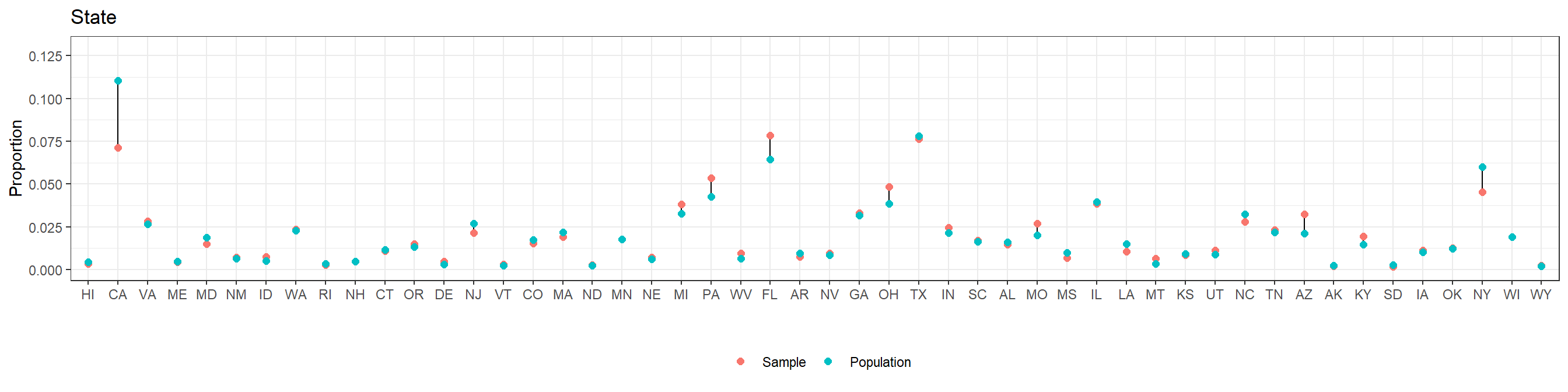
In the previous steps we have obtained a 5,000-person sample from the CCES survey and also generated a poststratification table using census data. As a first exploratory step, we will check if the frequencies for the different levels of the factors considered in the CCES data are similar to the frequencies reported in the census. If this was not the case, we will start suspecting some degree of nonresponse bias in the CCES survey.

For clarity, the levels in the plots follow their natural order in the case of age and education, ordering the others by the approximate proportion of Republican support.

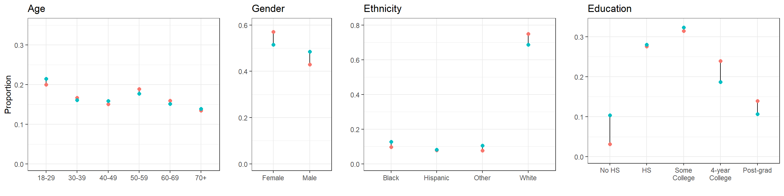
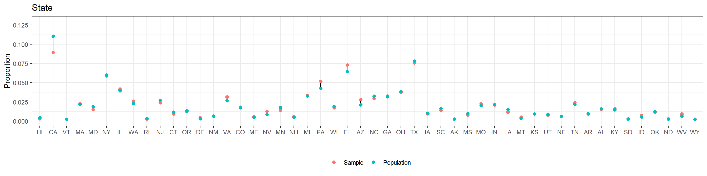
We see that our 5,000-participant CCES sample does not differ too much from the target population according to the American Community Survey. This should not be surprising, as the CCES intends to use a representative sample.

In general, we recommend checking the differences between the sample and the target population. In this case, the comparison has been based on the factors that are going to be used in MRP. However, even if some non-response bias existed for any of these factors MRP would be able to adjust for it, as we will see more in detail in subsection 4. Therefore, it may be especially important to compare the sample and target population with respect to the variables that are not going to be used in MRP – and, consequently, where we will not be able to correct any outcome measure bias due to differential non-response in these non-MRP variables.

1.2 First stage: Estimating the Individual-Response Model

The first stage is to use a multilevel logistic regression model to predict the outcome measure based on a set of factors. Having a plausible model to predict opinion is central for MRP to work well.

The model we use in this example is described below. It includes varying intercepts for age, ethnicity, education, and state, where the variation for the state intercepts is in turn influenced by the region effects (coded as indicator variables) and the Republican vote share in the 2016 election. As there are only two levels for gender, it is preferable to model it as a predictor for computational efficiency. Additionally, we include varying intercepts for the interaction between gender and ethnicity, education and age, and education and ethnicity (see Ghitza and Gelman (2013) for an in-depth discussion on interactions in the context of MRP).

\[ Pr(y_i = 1) = logit^{-1}( \alpha_{\rm s[i]}^{\rm state} + \alpha_{\rm a[i]}^{\rm age} + \alpha_{\rm r[i]}^{\rm eth} + \alpha_{\rm e[i]}^{\rm educ} + \beta^{\rm male} \cdot {\rm Male}_{\rm i} + \alpha_{\rm g[i], r[i]}^{\rm male.eth} + \alpha_{\rm e[i], a[i]}^{\rm educ.age} + \alpha_{\rm e[i], r[i]}^{\rm educ.eth} ) \] where:

\[ \begin{aligned} \alpha_{\rm s}^{\rm state} &\sim {\rm normal}(\gamma^0 + \gamma^{\rm south} \cdot {\rm South}_{\rm s} + \gamma^{\rm northcentral} \cdot {\rm NorthCentral}_{\rm s} + \gamma^{\rm west} \cdot {\rm West}_{\rm s} \\ & \quad + \gamma^{\rm repvote} \cdot {\rm RepVote}_{\rm s}, \sigma^{\rm state}) \textrm{ for s = 1,...,50}\\ \alpha_{\rm a}^{\rm age} & \sim {\rm normal}(0,\sigma^{\rm age}) \textrm{ for a = 1,...,6}\\ \alpha_{\rm r}^{\rm eth} & \sim {\rm normal}(0,\sigma^{\rm eth}) \textrm{ for r = 1,...,4}\\ \alpha_{\rm e}^{\rm educ} & \sim {\rm normal}(0,\sigma^{\rm educ}) \textrm{ for e = 1,...,5}\\ \alpha_{\rm g,r}^{\rm male.eth} & \sim {\rm normal}(0,\sigma^{\rm male.eth}) \textrm{ for g = 1,2 and r = 1,...,4}\\ \alpha_{\rm e,a}^{\rm educ.age} & \sim {\rm normal}(0,\sigma^{\rm educ.age}) \textrm{ for e = 1,...,5 and a = 1,...,6}\\ \alpha_{\rm e,r}^{\rm educ.eth} & \sim {\rm normal}(0,\sigma^{\rm educ.eth}) \textrm{ for e = 1,...,5 and r = 1,...,4}\\ \end{aligned} \]

Where:

• \(\alpha_{\rm a}^{\rm age}\): The effect of subject \(i\)’s age on the probability of supporting the statement.

• \(\alpha_{\rm r}^{\rm eth}\): The effect of subject \(i\)’s ethnicity on the probability of supporting the statement.

• \(\alpha_{\rm e}^{\rm educ}\): The effect of subject \(i\)’s education on the probability of supporting the statement.

• \(\alpha_{\rm s}^{\rm state}\): The effect of subject \(i\)’s state on the probability of supporting the statement. As we have a state-level predictor (the Republican vote share in the 2016 election), we need to build another model in which \(\alpha_{\rm s}^{\rm state}\) is the outcome of a linear regression with an expected value determined by an intercept \(\gamma^0\), the effect of the region coded as indicator variables (with Northeast as the baseline level), and the effect of the Republican vote share \(\gamma^{\rm demvote}\).

• \(\beta^{\rm male}\): The average effect of being male on the probability of supporting abortion. We could have used a similar formulation as in the previous cases (i.e. \(\alpha_{\rm g}^{\rm gender} \sim N(0, \sigma^{\rm gender})\)), but having only two levels (i.e. male and female) can create some estimation problems.

• \(\alpha_{\rm e,r}^{\rm male.eth}\) and \(\alpha_{\rm e,r}^{\rm educ.age}\): In the survey literature it is common practice to include these two interactions.

• \(\alpha_{\rm e,r}^{\rm educ.eth}\): In the next section we will explore public opinion on required abortion coverage at the different levels of education and ethnicity. It is, therefore, a good idea to also include this interaction.

Readers without a background in multilevel modeling may be surprised to see this formulation. Why are we using terms such as \(\alpha_{\rm eth}^{\rm eth}\) instead of the much more common method of creating an indicator variable for each state (e.g. \(\beta^{\rm white} \cdot {\rm White}_{i} + \beta^{\rm black} \cdot {\rm Black}_{i} + ...\))? The answer is that this approach allows to share information between the levels of each variable (e.g. different ethnicities), preventing levels with less data from being too sensitive to the few observed values. For instance, it could happen that we only surveyed ten Hispanics, and that none of them turned out to agree that employers should be able to decline abortion coverage in insurance plans. Under the typical approach, the model would take this data too seriously and consider that Hispanics necessarily oppose this statement (i.e. \(\beta^{\rm hispanic} = - \infty\)). We know, however, that this is not the case. It may be that Hispanics are less likely to support the statement, but from such a small sample size it is impossible to know. What the multilevel model will do is to partially pool the varying intercept for Hispanics towards the average accross all ethnicities (i.e. in our model, the average across all ethnicities is fixed at zero), making it negative but far from the unrealistic negative infinity. This pooling will be data-dependent, meaning that it will pool the varying intercept towards the average more strongly the smaller the sample size in that level. In fact, if the sample size for a certain level is zero, the estimate varying intercept would be the average coefficient for all the other levels. We recommend Gelman and Hill (2006) for an introduction to multilevel modeling.

The rstanarm package allows the user to conduct complicated regression analyses in Stan with the simplicity of standard formula notation in R. stan_glmer(), the function that allows to fit generalized linear multilevel models, uses the same notation as the lme4 package (see documentation here). That is, we specify the varying intercepts as (1 | group) and the interactions are expressed as (1 | group1:group2), where the : operator creates a new grouping factor that consists of the combined levels of the two groups (i.e. this is the same as pasting together the levels of both factors). However, this syntax only accepts predictors at the individual level, and thus the two state-level predictors must be expanded to the individual level (see [p. 265-266]Gelman and Hill (2006)). Notice that:

\[ \begin{aligned} \alpha_{\rm s}^{\rm state} &\sim {\rm normal}(\gamma^0 + \gamma^{\rm south} \cdot {\rm South}_{\rm s} + \gamma^{\rm northcentral} \cdot {\rm NorthCentral}_{\rm s} + \gamma^{\rm west} \cdot {\rm West}_{\rm s} + \gamma^{\rm repvote} \cdot {\rm RepVote}_{\rm s}, \sigma^{\rm state}) \\ &= \underbrace{\gamma^0}_\text{Intercept} + \underbrace{{\rm normal}(0, \sigma^{\rm state})}_\text{State varying intercept} + \underbrace{\gamma^{\rm south} \cdot {\rm South}_{\rm s} + \gamma^{\rm northcentral} \cdot {\rm NorthCentral}_{\rm s} + \gamma^{\rm west} \cdot {\rm West}_{\rm s} + \gamma^{\rm repvote} \cdot {\rm RepVote}_{\rm s}}_\text{State-level predictors expanded to the individual level} \end{aligned} \]

Consequently, we can then reexpress the model as:

\[ \begin{aligned} Pr(y_i = 1) =& logit^{-1}( \gamma^0 + \alpha_{\rm s[i]}^{\rm state} + \alpha_{\rm a[i]}^{\rm age} + \alpha_{\rm r[i]}^{\rm eth} + \alpha_{\rm e[i]}^{\rm educ} + \beta^{\rm male} \cdot {\rm Male}_{\rm i} + \alpha_{\rm g[i], r[i]}^{\rm male.eth} + \alpha_{\rm e[i], a[i]}^{\rm educ.age} + \alpha_{\rm e[i], r[i]}^{\rm educ.eth} + \gamma^{\rm south} \cdot {\rm South}_{\rm s} \\ &+ \gamma^{\rm northcentral} \cdot {\rm NorthCentral}_{\rm s} + \gamma^{\rm west} \cdot {\rm West}_{\rm s} + \gamma^{\rm repvote} \cdot {\rm RepVote}_{\rm s}) \end{aligned} \]

In the previous version of the model, \(\alpha_{\rm s[i]}^{\rm state}\) was informed by several state-level predictors. This reparametrization expands the state-level predictors at the individual level, and thus \(\alpha_{\rm s[i]}^{\rm state}\) now represents the variance introduced by the state adjusting for the region and 2016 Republican vote share. Similarly, \(\gamma^0\), which previously represented the state-level intercept, now becomes the individual-level intercept. The two parameterizations of the multilevel model are mathematically equivalent, and using one or the other is simply a matter of preference. The former one highlights the role that state-level predictos have in accounting for structured differences among the states, while the later is closer to the rstanarm syntax.

# Expand state-level predictors to the individual level
cces_df <- left_join(cces_df, statelevel_predictors_df, by = "state")

# Fit in stan_glmer
fit <- stan_glmer(abortion ~ (1 | state) + (1 | eth) + (1 | educ) + male +
                    (1 | male:eth) + (1 | educ:age) + (1 | educ:eth) +
                    repvote + factor(region),
  family = binomial(link = "logit"),
  data = cces_df,
  prior = normal(0, 1, autoscale = TRUE),
  prior_covariance = decov(scale = 0.50),
  adapt_delta = 0.99,
  refresh = 0,
  seed = 1010)

As a first pass to check whether the model is performing well, we must check that there are no warnings about divergences, failure to converge or tree depth. Fitting the model with the default settings produced a few divergent transitions, and thus we decided to try increasing adapt_delta to 0.99 and introducing stronger priors than the rstanarm defaults. After doing this, the divergences dissapeared. In the Computational Issues subsection we provide more details about divergent transitions and potential solutions.

print(fit)

## stan_glmer
##  family:       binomial [logit]
##  formula:      abortion ~ (1 | state) + (1 | eth) + (1 | educ) + male + (1 | 
##     male:eth) + (1 | educ:age) + (1 | educ:eth) + repvote + factor(region)
##  observations: 5000
## ------
##                         Median MAD_SD
## (Intercept)             -1.2    0.4  
## male                     0.3    0.1  
## repvote                  1.6    0.5  
## factor(region)Northeast -0.1    0.1  
## factor(region)South      0.2    0.1  
## factor(region)West      -0.1    0.1  
## 
## Error terms:
##  Groups   Name        Std.Dev.
##  state    (Intercept) 0.203   
##  educ:age (Intercept) 0.201   
##  educ:eth (Intercept) 0.084   
##  male:eth (Intercept) 0.222   
##  educ     (Intercept) 0.209   
##  eth      (Intercept) 0.374   
## Num. levels: state 50, educ:age 30, educ:eth 20, male:eth 8, educ 5, eth 4 
## 
## ------
## * For help interpreting the printed output see ?print.stanreg
## * For info on the priors used see ?prior_summary.stanreg

We can interpret the resulting model as follows:

• Intercept (\(\gamma^0\)): The global intercept corresponds to the expected outcome in the logit scale when having all the predictors equal to zero. In this case, this does not have a clear interpretation, as it is then influenced by the varying intercepts for state, age, ethnicity, education, and interactions. Furthermore, it corresponds to the impractical scenario of someone in a state with zero Republican vote share.

• male (\(\beta^{\rm male}\)): The median estimate for this coefficient is 0.3, with a standard error (measured using the Mean Absolute Deviation) of 0.1. Using the divide-by-four rule (Gelman, Hill, and Vehtari (2020), Chapter 13), we see that, adjusting for the other covariates, males present up to a 7.5% \(\pm\) 2.5% higher probability of supporting the right of employers to decline coverage of abortions relative to females.

• repvote (\(\gamma^{\rm repvote}\)): As the scale of repvote was between 0 and 1, this coefficient corresponds to the difference in probability of supporting the statement between someone that was in a state in which no one voted Republican to someone whose state voted all Republican. This is not reasonable, and therefore we start by dividing the median coefficient by 10. Doing this, we consider a difference of a 10% increase in Republican vote share. This means that we expect that someone from a state with a 55% Republican vote share has approximately \(\frac{1.6}{10}/4 = 4\%\) (\(\pm 12.5\%\)) higher probability of supporting the statement relative to another individual with similar characteristics from a state in which Republicans received 45% of the vote.

• regionSouth (\(\gamma^{\rm south}\)): According to the model, we expect that someone from a state in the south has, adjusting for the other covariates, up to a 0.2/4 = 5% (\(\pm\) 2%) higher probability of supporting the statement relative to someone from the Northeast, which was the baseline category. The interpretation for regionNorthCentral and regionWest is similar.

• Error terms (\(\sigma^{\rm state}\), \(\sigma^{\rm age}\), \(\sigma^{\rm eth}\), \(\sigma^{\rm educ}\), \(\sigma^{\rm male.eth}\), \(\sigma^{\rm educ.age}\), \(\sigma^{\rm educ.eth}\)): Remember that the intercepts for the different levels of state, age, ethnicity, education, and the specified interactions are distributed following a normal distribution centered at zero and with a standard deviation that is estimated from the data. The Error terms section gives us the estimates for these group-level standard deviations. For instance, \(\alpha_{\rm r}^{\rm ethnicity} \sim {\rm normal}(0, \sigma^{\rm ethnicity})\), where the median estimate for \(\sigma^{\rm ethnicity}\) is 0.374. In other words, the variyng intercepts for the different ethnicity groups have a standard deviation that is estimated to be 0.374 on the logit scale, or 0.374/4 = 0.094 on the probability scale. In some cases, we may also want to check the intercepts corresponding to the individual levels of a factor. In rstanarm, this can be done using fit$coefficients. For instance, the median values for the varying intercepts of race are \(\alpha^{\rm eth}_{r = {\rm White}}\) = 0.15, \(\alpha^{\rm eth}_{r = {\rm Black}}\) = -0.28, \(\alpha^{\rm eth}_{r = {\rm Hispanic}}\) = 0.03, \(\alpha^{\rm eth}_{r = {\rm Other}}\) = 0.08.

1.3 Second Stage: Poststratification

Estimation at the national level

Currently, all we have achieved is a model that, considering certain factor-type predictors, predicts support for providing employers with the option to decline abortion coverage. To go from this model to a national or subnational estimate, we need to weight the model predictions for the different subgroups by the actual frequency of these subgroups. This idea can be expressed as:

\[ \theta^{MRP} = \frac{\sum N_j \theta_j}{\sum N_j} \]

where \(\theta^{MRP}\) is the MRP estimate, \(\theta_{\rm j}\) corresponds to the model estimate for a specific subgroup defined in a cell of the poststratification table (e.g. young Hispanic men with a High School diploma in Arkansas), and \(N_{\rm j}\) corresponds to the number of people in that subgroup. For a more in-depth review of poststratification, see Chapter 13 of Gelman, Hill, and Vehtari (2020).

The values of \(\theta_{j}\) for the different subgroups can be obtained with the posterior_epred() function. Of course, as stan_glmer() performs Bayesian inference, \(\theta_{j}\) for any given subgroup will not be a single point estimate but a vector of posterior draws.

# Expand state level predictors to the individual level
poststrat_df <- left_join(poststrat_df, statelevel_predictors_df, by = "state")

# Posterior_epred returns the posterior estimates for the different subgroups stored in the
# poststrat_df dataframe. 
epred_mat <- posterior_epred(fit, newdata = poststrat_df, draws = 1000)
mrp_estimates_vector <- epred_mat %*% poststrat_df$n / sum(poststrat_df$n)
mrp_estimate <- c(mean = mean(mrp_estimates_vector), sd = sd(mrp_estimates_vector))
cat("MRP estimate mean, sd: ", round(mrp_estimate, 3))

## MRP estimate mean, sd:  0.433 0.007

posterior_epred() returns a matrix \(P\) with \(D\) rows and \(J\) columns, where \(D\) corresponds to the number of draws from the posterior distribution (in this case 1000, as we specified draws = 1000) and \(J\) is the number of subgroups in the poststratification table (i.e. 12,000). This matrix, which was called epred_mat in our code, is multiplied by a vector \(k\) of length \(J\) that contains the number of people in each subgroup of the poststratification table. This results in a vector of length \(D\) that is then divided by the total number of people considered in the poststratification table, a scalar which is calculated by adding all the values in \(k\).

\[\theta^{MRP} = \frac{P \times k}{\sum_j^J k_j}\]

The end result is a vector that we call \(\theta^{MRP}\), and which contains \(D\) estimates for the national-level statement support.

We can compare these results to the 5,000-person unadjusted sample estimate:

## Unadjusted 5000-respondent survey mean, sd:  0.431 0.007

Additionally, we compare with the population support estimated by the full CCES with close to 60,000 participants:

## Unadjusted 60,000-respondent survey mean, sd:  0.434 0.002

In general, we see that both the unadjusted sample estimate and the MRP estimate are quite close to the results of the full survey. In other words, MRP is not providing a notable advantage against the unadjusted sample national estimates. However, it is important to clarify that we were somewhat lucky in obtaining this result as a product of using data from the CCES, a high quality survey that intends to be representative (and appears to be, at least with respect to the variables considered in our poststratification table). Many real-world surveys are not as representative relative to the variables considered in the poststratification step, and in these cases MRP will help correcting the biased estimates from the unadjusted survey. We will see an example of this in section 4, where we exemplify how MRP adjusts a clearly biased sample.

Estimation for subnational units

As we mentioned, small area estimation is one of the main applications of MRP. In this case, we will get an estimate of the support for employer’s right to decline coverage of abortions per state:

\[ \theta_s^{MRP} = \frac{\sum_{j \in s} N_j \theta_j}{\sum_{j \in s} N_j} \]

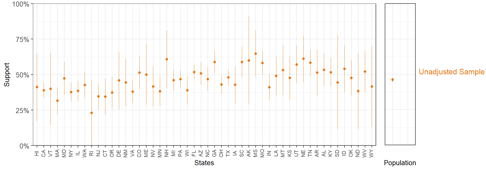
We start visualizing the estimates by state from the unadjusted 5,000-person sample. Again, the states are ordered by Republican vote in the 2016 election, and therefore we expect that statement support to follow an increasing trend.

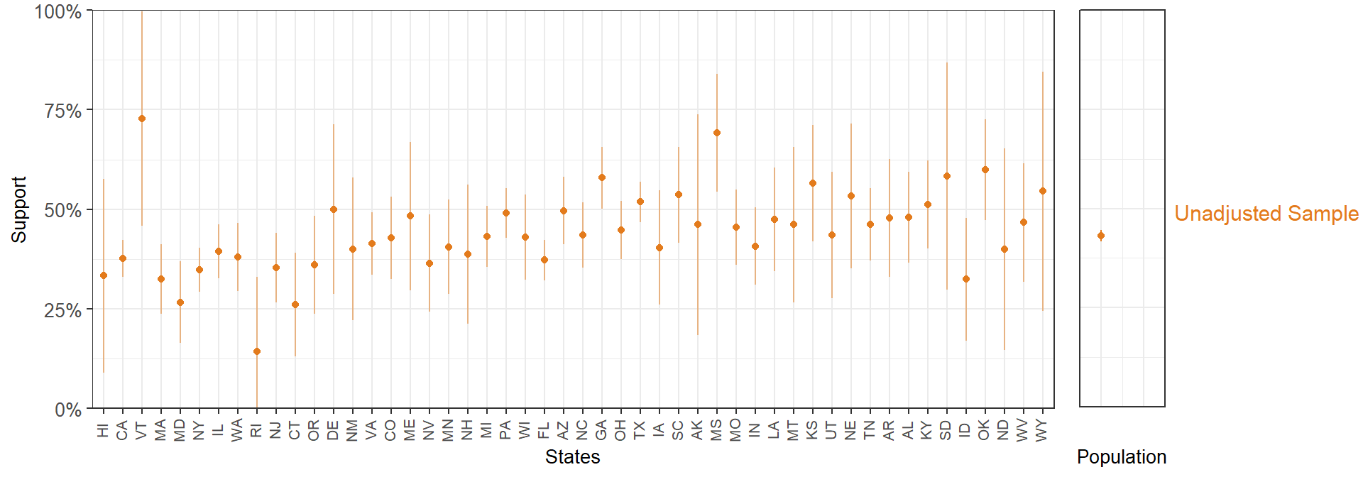
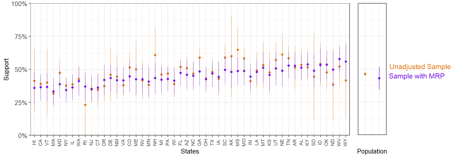
In states with small samples, we see considerably wide 95% confidence intervals. We can add the MRP-adjusted estimates to this plot.

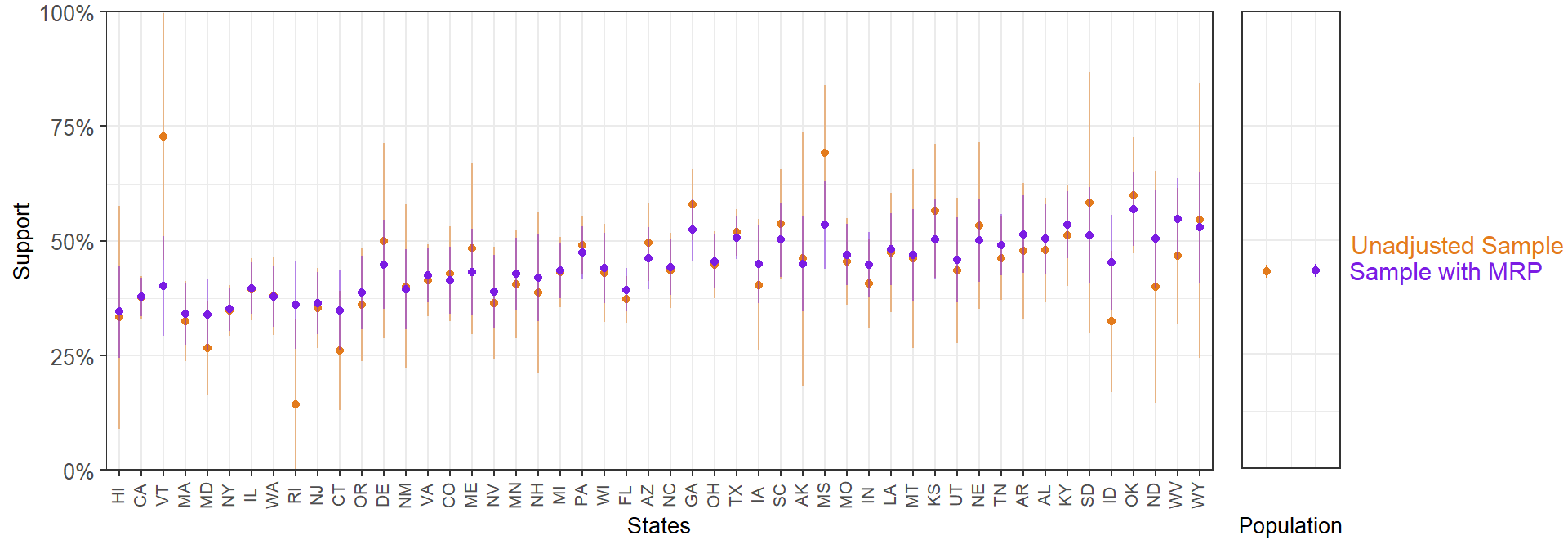
In general, MRP produces less extreme values by partially pooling information across the factor levels. To illustrate this, we can compare the sample and MRP estimates with the results form the full 60,000-respondent CCES. Of course, in any applied situation we would be using the data from all the participants, but as we took a 5,000 person sample the full 60,000-respondent survey serves as a reference point.

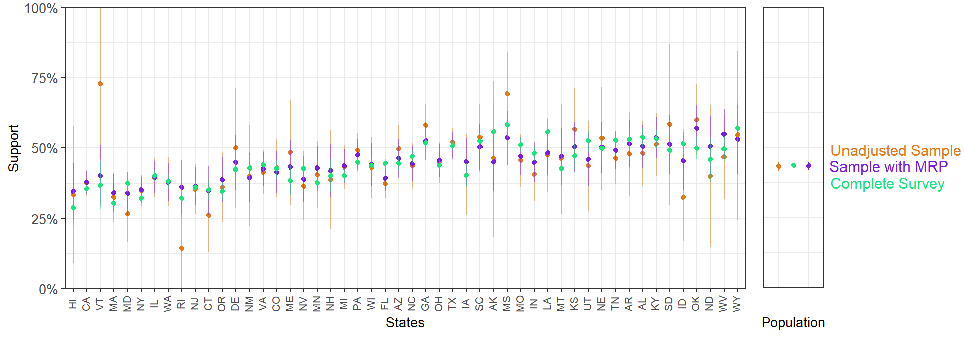
Overall, the MRP estimates are closer to the full survey estimates. This is particularly clear for the states with a smaller sample size.

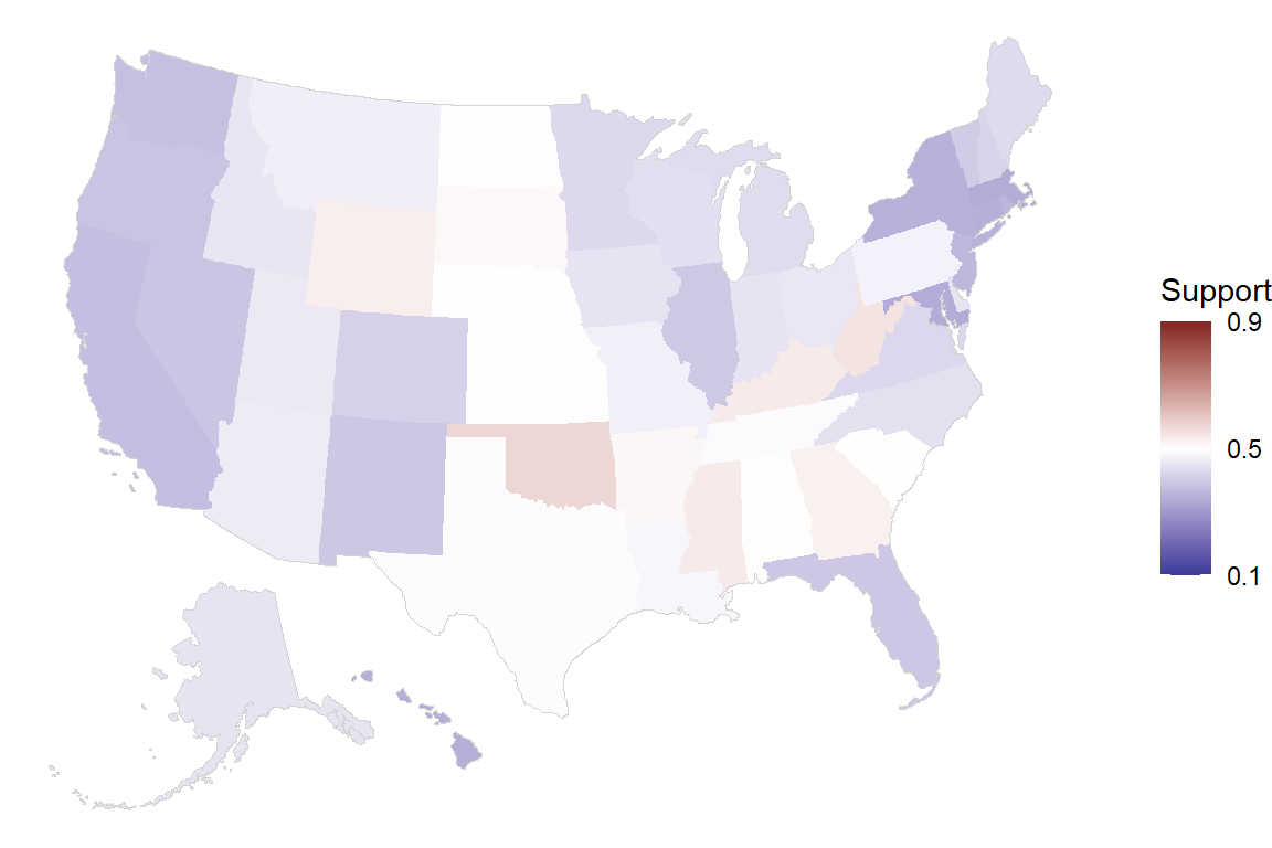
As a final way of presenting the MRP estimates, we can plot them on a US map. The symmetric color range goes from 10% to 90% support, as this scale allows for comparison with the other maps. However, the MRP estimates for statement support are concentrated in a relatively small range, which makes the colors appear muted.

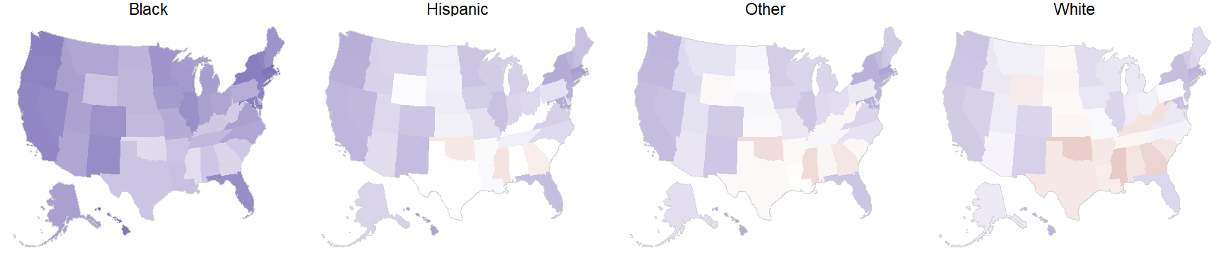
Estimation for subgroups within subnational units

MRP can also be used to obtain estimates for more complex cases, such as subgroups within states. For instance, we can study support for declining coverage of abortions by state and ethnicity within state. For clarity, we order the races according to their support for the statement.

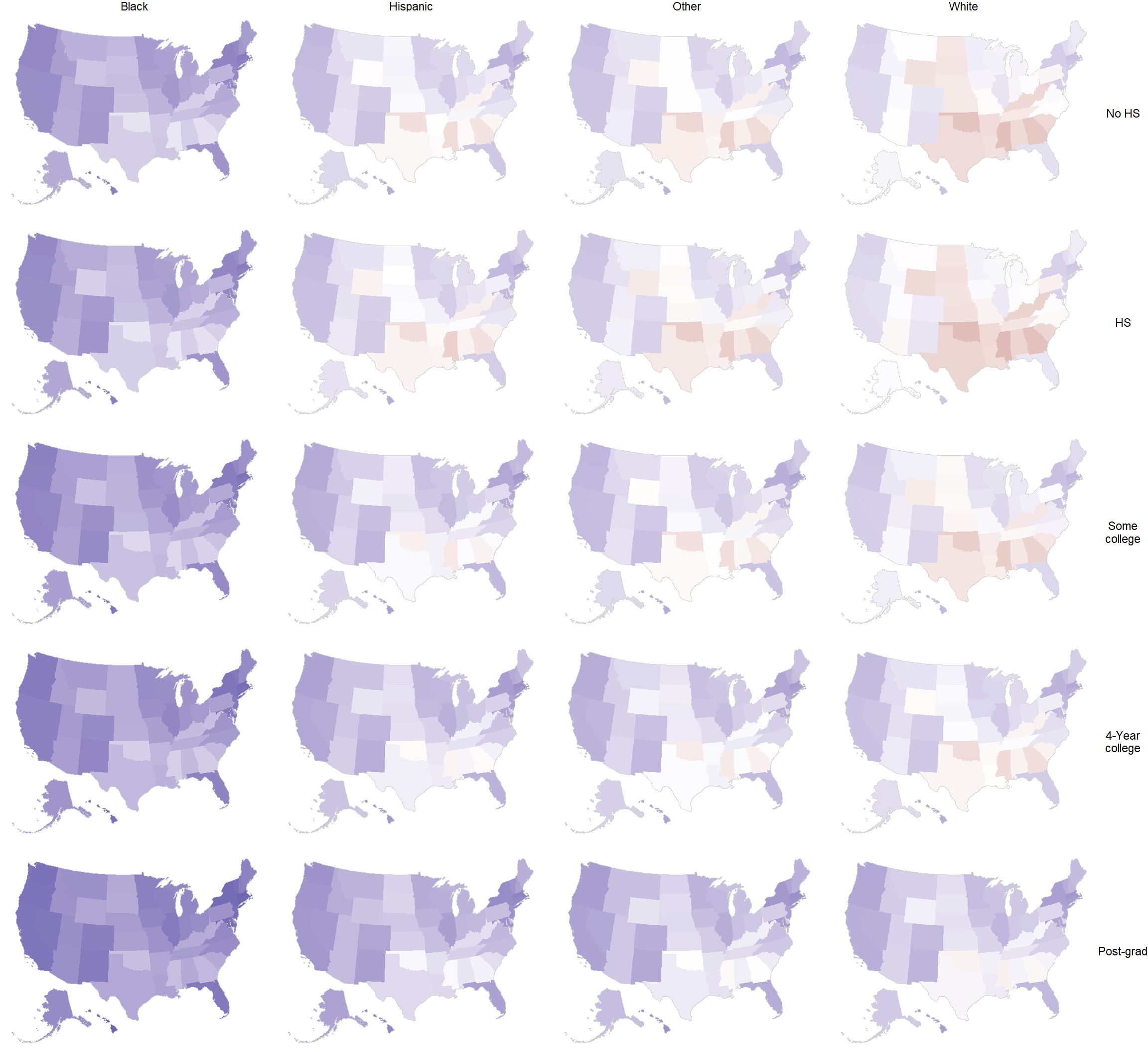
Similarly, we can look at the outcome in ethnicity-education subgroups by state.

1.4 Adjusting for Nonrepresentative Surveys

We have already introduced that MRP is an effective statistical adjustment method to correct for differences between the sample and target population for a set of key variables. We start this second example by obtaining an artificially nonrepresentative sample that gives more weight to respondents that are older, male, and from Republican states.

set.seed(1010)

# We add the state-level predictors to cces_all_df
cces_all_df <- left_join(cces_all_df, statelevel_predictors_df, by = "state")

# We take a sample from cces_all_df giving extra weight to respondents that are older, male, 
# and from Republican states.
cces_biased_df <- cces_all_df %>% 
  sample_n(5000, weight = I(5*repvote + (age=="18-29")*0.5 + (age=="30-39")*1 + 
                              (age=="40-49")*2 + (age=="50-59")*4 + 
                              (age=="60-69")*6 + (age=="70+")*8 + (male==1)*20 + 
                              (eth=="White")*1.05))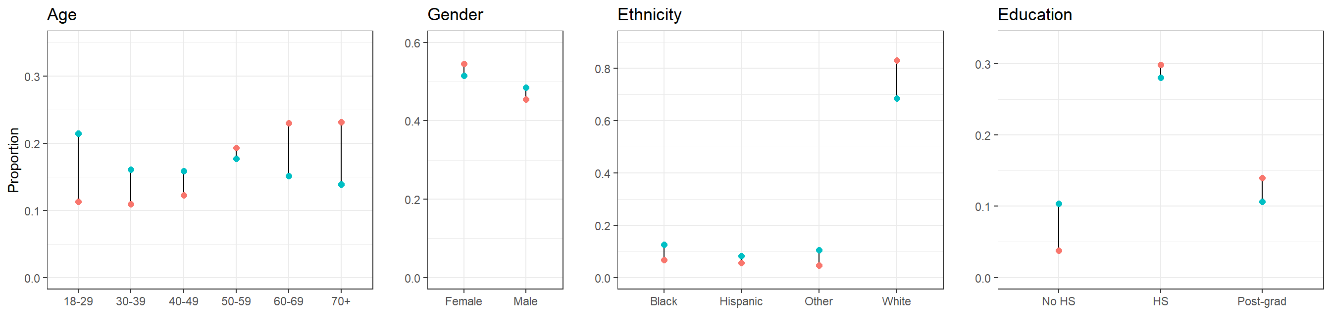

fit <- stan_glmer(abortion ~ (1 | state) + (1 | eth) + (1 | educ) + (1 | age) + male +
                    (1 | male:eth) + (1 | educ:age) + (1 | educ:eth) +
                    repvote + factor(region),
  family = binomial(link = "logit"),
  data = cces_biased_df,
  prior = normal(0, 1, autoscale = TRUE),
  prior_covariance = decov(scale = 0.50),
  adapt_delta = 0.99,
  refresh = 0,
  seed = 1010)

As expected, our remarkably nonrepresentative sample produces estimates that are lower than what we obtained by using a random sample in the previous section.

MRP seems to partially correct for the nonrepresentative sample:

Lastly, we see how the MRP national and subnational estimates based on the nonrepresentative sample are, overall, much closer to the 60,000-person survey than the biased unadjusted sample estimates.

1.5 Practical Considerations

Census incompletness and uncertainty

There are two main problems we can encounter when dealing with census data.

• It is possible that some variables that we may want to use for poststratification are not available. For instance, party ID is not registered in the US census and ethnicity is not registered in the French census. This additional information can be included in the poststratification table based on other (generally smaller) surveys that contain these variables.

• A great number of demogaphic-geographic combinations can require a large poststratification table, which in turn can result in unreliable census estimates. The American Community Survey we use in this case study does not only provide estimates of the actual figures that would have been obtained if the entire population was sampled, it also includes a measure of uncertainty around these estimates. Ideally, this uncertainty should be taken into account in the poststratification. For simplicity, this introduction has skipped this step, but this could mean the MRP-based estimates present an underestimated uncertainty.

Nonreponse and missing data

We have seen that MRP is a method that can mitigate potential biases in the sample, but it is not a substitute for a better data collection effort that tries to minimize systematic nonresponse patterns.

Model complexity

MRP depends upon the use of a regularized model (i.e. that prevents overfitting by limiting its complexity). Different approaches can be used for this goal (e.g. non-multilevel regression, random forests, or a neural network; see Bisbee (2019) for an implementation that uses Bayesian Additive Regression Trees and Ornstein (2020) for an ensemble of predictive models), but there are several advantages of using a Bayesian multilevel model. First, the multilevel structure allows for partially pooling information across different levels of a factor, which can be crucial when dealing with certain levels with few samples. Second, the Bayesian approach propagates uncertainty across the modeling, and thus gives more realistic confidence intervals.

Apart from selecting the demogaphic-geographic categories included in the poststratification table, there are several decisions the modeler should make. As we have already mentioned, adding relevant state-level predictors to the model often improves results, particularly when we have few data about some states. The inclusion of interactions can also be benefitial, especially when studying subgroups within subgroups (e.g. demographic subgroups within states; Ghitza and Gelman (2013)). Lastly, the use of structured priors can also serve to reduce both bias and variance by sharing information across the levels of a factor (Gao et al. (2020)).

Empty cells in the poststratification table

It is very frequent that some of the cells in the poststratification table are empty, meaning that there are not anyone that fulfills some specific combination of factors. For instance, in a given poststratification table we might find that there can be no people younger than 20, without a high school degree, and earning more than $500,000 a year in a particularly small state. In our example, we made sure that all the cells in the poststratification table were present even if the weight of that cell was zero, but this was only for illustrative purposes.

Subnational units not represented in the survey

It is fairly common for small-sample surveys not to include anyone from a particular subnational unit. For instance, a small national survey in the US may not include any participant from Wyoming. An important advantage of MRP is that we can still produce estimates for this state using the information from the participants in other states. Going back to the first parametrization of the multilevel model that we presented, \(\alpha^{\rm state}_{\rm s = Wyoming}\) will be calculated based on the region and Republican voteshare of the 2016 – even in the abscence of information about the effect of residing in Wyoming specifically. As we have already explained, including subnational-level predictors is always recommended, particularly considering that data at the subnational level is easy to obtain in many cases. However, when dealing with subnational units that are not represented in our survey these predictors become even more central, as they are able to capture structured differences among the states and therefore allow for more precise estimation in the missing subnational areas.

Computational issues

Stan uses Hamiltonian Monte Carlo to explore the posterior distribution. In some cases, the geometry of the posterior distribution is too complex, making the Hamiltonian Monte Carlo “diverge”. This produces a warning indicating the presence of divergent transitions after warmup, something that implies the model could present biased estimates (see Betancourt (2017) for more details). Usually, a few divergent transitions do not indicate a serious problem. There are, in any case, three potential solutions to this problem that do not involve reformulating the model: (i) a non-centered parametization; (ii) increasing the adapt_delta parameter; and (iii) including stronger priors. Fortunately we don’t have to worry about (i), as rstanarm already provides a non-centered parametization for the model. Therefore, we can focus on the other two.

1. Exploring the posterior distribution is somewhat similar as cartographing a mountainous terrain, and a divergent transition is similar to falling down a very steep slope, with the consequence of not being able to correctly map that area. In this analogy, what the cartographer could do is moving through the steep slope giving smaller steps to avoid falling. In Stan, the step size is set up automatically, but we can change a parameter called adapt_delta that controls the step size. By default we have that adapt_delta = .95, but we can increase that number to make Stan take smaller steps, which should reduce the number of divergent transitions. The maximum value we can set for adapt_delta is close (but necessarely less than) 1, with the downside that an increase implies a somewhat slower exploration of the posterior distribution. Usually, an adapt_delta = 0.99 works well if we only have a few divergent transitions.

2. However, there are cases in which increasing adapt_delta is not sufficient, and divergent transitions still occur. In this case, introducing weakly informative priors can be extremelly helpful. Although rstanarm provides by default weakly informative priors, in most applications these tend to be too weak. By using more reasonable priors, we make the posterior distribution easier to explore.

   • The priors for the scaled coefficients are \({\rm normal}(0, 2.5)\). When the coefficients are not scaled, rstanarm will automatically adjust the scaling of the priors as detailed in the prior vignette. In most cases, and particularly when we find computational issues, it is reasonable to give stronger priors on the scaled coefficients such as \({\rm normal}(0, 1)\).
   • Multilevel models with multiple group-level standard deviation parameters (e.g. \(\sigma^{\rm age}\), \(\sigma^{\rm eth}\), \(\sigma^{\rm educ.eth}\), etc.) tend to be hard to estimate and sometimes present serious computational issues. The default prior for the covariance matrix is decov(reg. = 1, conc. = 1, shape = 1, scale = 1). However, in a varying-intercept model such as this one (i.e. with structure (1 | a) + (1 | b) + ... + (1 | n)) the group-level standard deviations are independent of each other, and therefore the prior is simply a gamma distribution with some shape and scale. Consequently, decov(shape = 1, scale = 1) implies a weakly informative prior \({\rm Gamma(shape = 1, scale = 1)} = {\rm Exponential(scale = 1)}\) on each group-level standard deviation. This is too weak in most situations, and using something like \({\rm Exponential(scale = 0.5)}\) can be crucial for stabilizing computation.

Therefore, something like this has much fewer chances of running into computational issues than simply leaving the defaults:

fit <- stan_glmer(abortion ~ (1 | state) + (1 | eth) + (1 | educ) + (1 | age) + male + 
                    (1 | male:eth) + (1 | educ:age) + (1 | educ:eth) + 
                    repvote + factor(region),
  family = binomial(link = "logit"),
  data = cces_df,
  prior = normal(0, 1, autoscale = TRUE),
  prior_covariance = decov(scale = 0.50),
  adapt_delta = 0.99,
  refresh = 0,
  seed = 1010)

More details about divergent transitions can be found in the Brief Guide to Stan’s Warnings and in the Stan Reference Manual. More information and references about priors can be found in the Prior Choice Recommendations Wiki.

1.6 Appendix: Downloading and Processing Data

1.6.1 CCES

The 2018 CCES raw survey data can be downloaded from the CCES Dataverse via this link; by default the downloaded filename is called cces18_common_vv.csv.

Every MRP study requires some degree of data wrangling in order to make the factors in the survey of interest match the factors available in census data and other population-level surveys and census. Here we use the R Tidyverse to process the survey data so that it aligns with the postratification table. Because initial recoding errors are fatal, it is important to check that each step of the recoding process produces expected results, either by viewing or summarizing the data. Because the data is all tabular data, we use the utility function head to inspect the first few lines of a dataframe before and after each operation.

First, we examine the contents of the data as downloaded, looking only at those columns which provide the demographic-geographic information of interest. In this case, these are labeled as inputstate, gender, birthyr, race, and educ.

cces_all <- read_csv("data_public/chapter1/data/cces18_common_vv.csv.gz")

## Rows: 60000 Columns: 526
## -- Column specification ------------------------------------------------------------------------------------------------
## Delimiter: ","
## chr (165): race_other, CC18_354a_t, CC17_3534_t, CC18_351_t, CC18_351a_t, CC18_351b_t, CC18_351c_t, CC18_352_t, CC18...
## dbl (359): caseid, commonweight, commonpostweight, vvweight, vvweight_post, tookpost, CCEStake, birthyr, gender, edu...
## lgl   (2): multrace_97, multrace_99
## 
## i Use `spec()` to retrieve the full column specification for this data.
## i Specify the column types or set `show_col_types = FALSE` to quiet this message.

inputstate	gender	birthyr	race	educ
24	2	1964	5	4
47	2	1971	1	2
39	2	1958	1	3
6	2	1946	4	6
21	2	1972	1	2
4	2	1995	1	1

As we have seen, it is crucial that the geography and demographics for the survery must match the geography and demographics in the poststratification table. If there is not a direct one-to-one relationship between the survey and the population data, the survey data must be recoded until a clean mapping exists. We write R functions to encapsulate the recoding steps.

We start considering the geographic information. Both the CCES survey and the US Census data use numeric FIPS codes to record state information. We can use R factors to map FIPS codes to the standard two-letter state name abbreviations. Because both surveys use this encoding, we make this into a reusable function recode_fips.

# Note that the FIPS codes include the district of Columbia and US territories which
# are not considered in this study, creating some gaps in the numbering system.
state_ab <- datasets::state.abb
state_fips <- c(1,2,4,5,6,8,9,10,12,13,15,16,17,18,19,20,21,22,23,24,25,26,27,28,29,30,
                31,32,33,34,35,36,37,38,39,40,41,42,44,45,46,47,48,49,50,51,53,54,55,56)
recode_fips <- function(column) {
    factor(column, levels = state_fips, labels = state_ab)
}

Secondly, we recode the demographics in order for them to be compatible with the American Community Survey data. In some cases this requires changing the levels of a factor (e.g. ethnicity) and in others we may need ot split a continous variable into different intervals (e.g. age). clean_cces uses the recode_fips function defined above to clean up the states. By default, the clean_cces functions drops rows where there is non-response in any of the considered factors or in the outcome variable; if this information is not missing at random, this introduces (more) bias into our survey.

# Recode CCES
clean_cces <- function(df, remove_nas = TRUE){
  
  ## Abortion -- dichotomous (0 - Oppose / 1 - Support)
  df$abortion <- abs(df$CC18_321d-2)
  
  ## State -- factor
  df$state <- recode_fips(df$inputstate)
  
  ## Gender -- dichotomous (coded as -0.5 Female, +0.5 Male)
  df$male <- abs(df$gender-2)-0.5
  
  ## ethnicity -- factor
  df$eth <- factor(df$race,
                   levels = 1:8,
                   labels = c("White", "Black", "Hispanic", "Asian", "Native American", 
                              "Mixed", "Other", "Middle Eastern"))
  df$eth <- fct_collapse(df$eth, "Other" = c("Asian", "Other", "Middle Eastern", 
                                             "Mixed", "Native American"))
  
  ## Age -- cut into factor
  df$age <- 2018 - df$birthyr
  df$age <- cut(as.integer(df$age), breaks = c(0, 29, 39, 49, 59, 69, 120), 
                labels = c("18-29","30-39","40-49","50-59","60-69","70+"),
                ordered_result = TRUE)
  
  ## Education -- factor
  df$educ <- factor(as.integer(df$educ), 
                    levels = 1:6, 
                    labels = c("No HS", "HS", "Some college", "Associates", 
                               "4-Year College", "Post-grad"), ordered = TRUE)
  df$educ <- fct_collapse(df$educ, "Some college" = c("Some college", "Associates"))  
  
  # Filter out unnecessary columns and remove NAs
  df <- df %>% select(abortion, state, eth, male, age, educ) 
  if (remove_nas){
    df <- df %>% drop_na()
  }
  
  return(df)
}

1.6.2 American Community Survey

We used the US American Community Survey to create a poststratification table. We will show two different (but equivalent) ways to do this.

Alternative 1: IPUMS

The Integrated Public Use Microdata Series (IPUMS) (Ruggles et al. (2020)) is a service run by the University of Minnesota that allows easy access to census and survey data. We focus on the IPUMS USA section, which preserves and harmonizes US census microdata, including the American Community Survey. Other researchers may be interested in IPUMS international, which contains census microdata for over 100 countries.

In order to create the poststratification table we took the following steps:

1. Register at IPUMS using the following link
2. On ipums.org, select IPUMS USA and then click on “Get Data”. This tool allows to easily select certain variables from census microdata using an intuitive point-and-click interface.

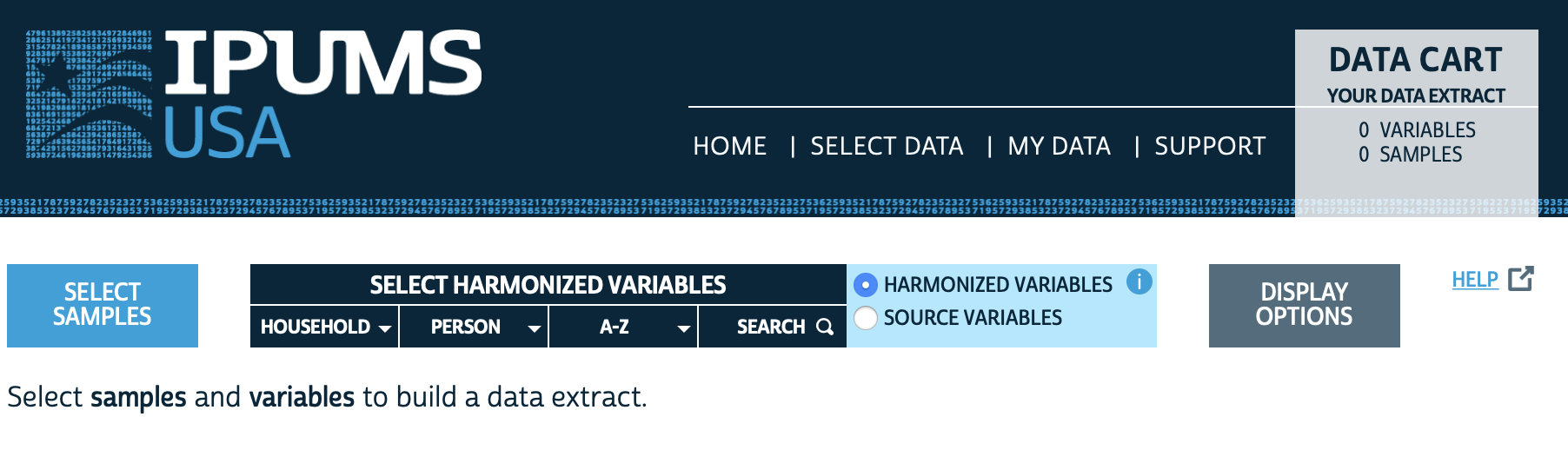
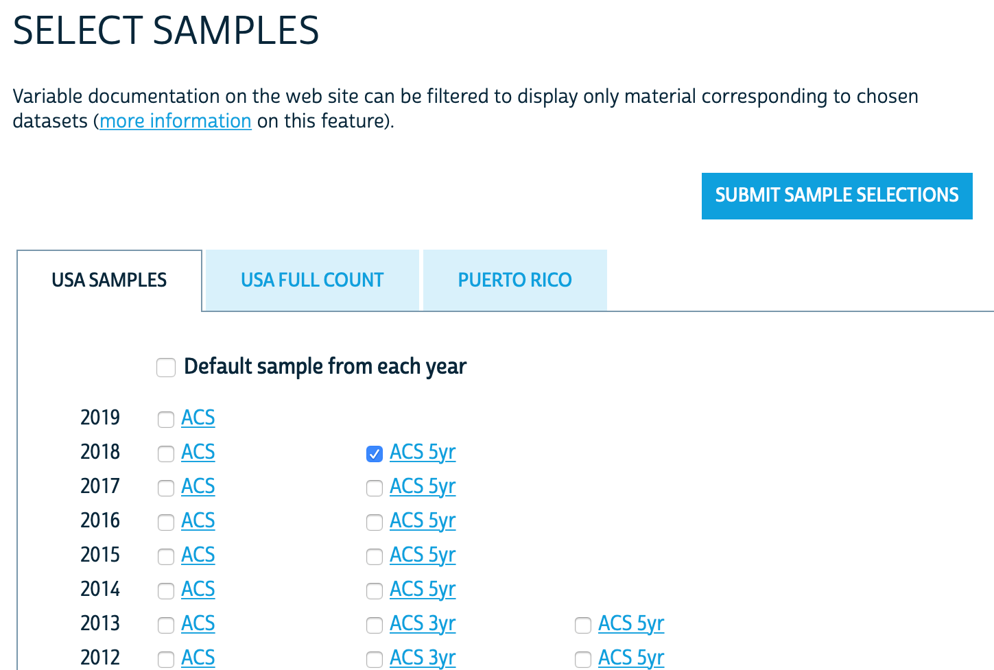
3. We first need to select a sample (i.e. the survey we want to use for the poststratification table) with a menu that is opened by clicking on the SELECT SAMPLES button shown above. In our case, we we will select the 2018 5-year ACS survey and then click on SUBMIT SAMPLE.

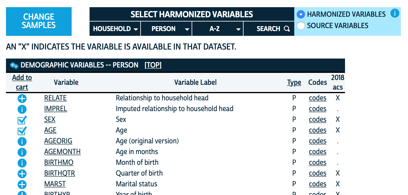
4. After selecting the sample we need to select the variables that will be included in our poststratification table. The multiple variables are conveniently categorized by HOUSEHOLD (household-level variables), PERSON (individual-level variables), and A-Z (alphabetically). For instance, clicking on PERSON > DEMOGRAPHIC displays the demographic variables, as shown below. Note that the rightmost column shows if that variable is available in the 2018 5-year ACS. Note that if you click on a certain variable IPUMS will provide a description and show the codes and frequencies. Based on the data available in your survey of interest, this is a useful tool to decide which variables to include in the poststratification table. In our case, we select:

• On PERSON > DEMOGRAPHIC select SEX and AGE
• On PERSON > RACE, ETHNICITY, AND NATIVITY select RACE, HISPAN, and CITIZEN
• On PERSON > EDUCATION select EDUC
• On HOUSEHOLD > GEOGRAPHIC select STATEFIP

6. We can review the variables we have selected by clicking on VIEW CART. This view also includes the ones which are automatically selected by IPUMS.

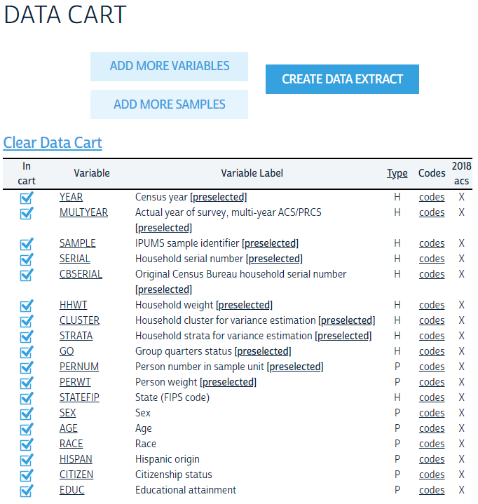
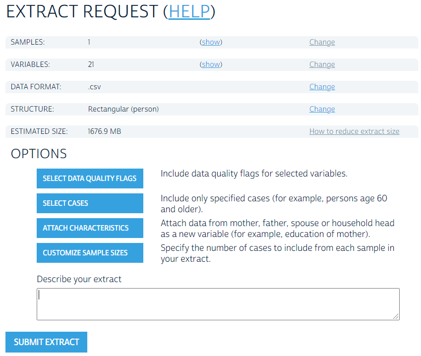
7. After reviewing these variables we should select CREATE DATA EXTRACT. By default the data format is a .dat with fixed-width text, but if we prefer we can change this to csv. After clicking SUBMIT EXTRACT the data will be generated. This can take a while, but you will receive an email when the file is ready for download.

7. Lastly, we download and preprocess the data. There are two main considerations:

   • Focus on the population of interest: We must take into account that the population of interest for the CCES survey, which only considers US citizens above 18 years of age, is different from the population reflected in the ACS. Therefore, we had to remove the cases of underages and non-citizens in the census data.

   • Match the levels of the two datasets: The levels of the variables in the poststratification table must match the levels of the variables in the CCES dataset. This required preprocessing the variables of the CCES and ACS in a way that the levels were compatible.

## Read data downloaded from IPUMS. This step can be slow, as the dataset is almost 1.5Gb
## (note: due to its size, this file is not included in the book repo)
temp_df <- read.csv('usa_00001.csv')

## Remove non-citizens
temp_df <- temp_df %>% filter(CITIZEN<3)

## State
temp_df$state <- temp_df$STATEFIP

## Gender
temp_df$male <- abs(temp_df$SEX-2)-0.5

## Ethnicity
temp_df$RACE <- factor(temp_df$RACE, 
                        levels = 1:9, 
                        labels = c("White", "Black", "Native American", "Chinese",
                                   "Japanese", "Other Asian or Pacific Islander", 
                                   "Other race, nec", "Two major races", 
                                   "Three or more major races"))
temp_df$eth <- fct_collapse(temp_df$RACE, 
                            "Other" = c("Native American", "Chinese", 
                                        "Japanese", "Other Asian or Pacific Islander", 
                                        "Other race, nec", "Two major races", 
                                        "Three or more major races"))
levels(temp_df$eth) <- c(levels(temp_df$eth), "Hispanic")
## add hispanic as ethnicity. This is done only for individuals that indicate being white 
# in RACE and of hispanic origin in HISPAN
temp_df$eth[(temp_df$HISPAN!=0) & temp_df$eth=="White"] <- "Hispanic"

## Age
temp_df$age <- cut(as.integer(temp_df$AGE), breaks = c(0, 17, 29, 39, 49, 59, 69, 120),
                   labels = c("0-17", "18-29","30-39","40-49","50-59","60-69","70+"),
                   ordered_result = TRUE)
# filter out underages
temp_df <- filter(temp_df, age!="0-17")
temp_df$age <- droplevels(temp_df$age)

## Education
# we need to use EDUCD (i.e. education detailed) instead of EDUC (i.e. general codes), as the
# latter does not contain enough information about whether high school was completed or not.
temp_df$educ <- cut(as.integer(temp_df$EDUCD), c(0, 61, 64, 100, 101, Inf), 
                    ordered_result = TRUE,
                    labels = c("No HS", "HS", "Some college", "4-Year College", "Post-grad"))

# Clean temp_df by dropping NAs and cleaning states with recode_fips
temp_df <- temp_df %>% drop_na(state, eth, male, age, educ, PERWT) %>% 
  select(state, eth, male, age, educ, PERWT) %>% filter(state %in% state_fips) %>% 
  mutate(state = recode_fips(state))
# Generate cell frequencies using groupby
poststrat_df <- temp_df %>%
  group_by(state, eth, male, age, educ, .drop = FALSE) %>% 
  summarise(n = sum(as.numeric(PERWT)))
# Write as csv
write.csv(poststrat_df, "poststrat_df.csv", row.names = FALSE)

If you use IPUMS in your project, don’t forget to cite it.

Alternative 2: ACS PUMS

Some researchers may prefer to access the 2018 5-year ACS data directly without using IPUMS, which makes the process less intuitive but also more reproducible. Additionally, this does not require creating an account, as the Public Use Microdata Sample (PUMS) from the ACS can be downloaded directly from the data repository. The repository contains two .zip files for each state: one for individual-level variables and other for household-level variables. All the variables considered in our analysis are available in the individual-level files, but we will also download and process the household-level variable income to show how this could be done.

# We start downloading all the zip files using wget. If you are using Windows you can download
# a pre-built wget from http://gnuwin32.sourceforge.net/packages/wget.htm
dir.create("poststrat_data/")
system('wget -O poststrat_data -e robots=off -nd -A "csv_*.zip" -R "index.html","csv_hus.zip",
"csv_pus.zip" https://www2.census.gov/programs-surveys/acs/data/pums/2018/5-Year/')

If this does not work, you can also access the data repository and download the files directly from your browser.

Once the data is downloaded, we process the .zip files for each state and then merge them together. IPUMS integrates census data accross different surveys, which results in different naming conventions and levels in some of the variables with respect to the PUMS data directly downloaded from the ACS repository. Therefore, the preprocessing steps is slightly different from the code shown above, but as the underlying data is the same we obtain an identical poststratification table.

list_states_abb <- datasets::state.abb
list_states_num <- rep(NA, length(list_states_abb))

list_of_poststrat_df <- list()

for(i in 1:length(list_states_num)){
  # Unzip and read household and person files for state i
  p_name <- paste0("postrat_data/csv_p", tolower(list_states_abb[i]),".zip")
  h_name <- paste0("postrat_data/csv_h", tolower(list_states_abb[i]),".zip")
  p_csv_name <- grep('\\.csv$', unzip(p_name, list=TRUE)$Name, ignore.case=TRUE, value=TRUE)
  temp_df_p_state <- fread(unzip(p_name, files = p_csv_name), header=TRUE, 
                           select=c("SERIALNO","ST","CIT","PWGTP","RAC1P","HISP","SEX",
                                    "AGEP","SCHL"))
  h_csv_name <- grep('\\.csv$', unzip(h_name, list=TRUE)$Name, ignore.case=TRUE, value=TRUE)
  temp_df_h_state <- fread(unzip(h_name, files = h_csv_name),
                         header=TRUE, select=c("SERIALNO","FINCP"))
  
  # Merge the individual and household level variables according to the serial number
  temp_df <- merge(temp_df_h_state, temp_df_p_state, by = "SERIALNO")

  # Update list of state numbers that will be used later
  list_states_num[i] <-  temp_df$ST[1]

  ## Filter by citizenship
  temp_df <- temp_df %>% filter(CIT!=5)

  ## State
  temp_df$state <- temp_df$ST

  ## Gender
  temp_df$male <- abs(temp_df$SEX-2)-0.5

  ## Tthnicity
  temp_df$RAC1P <- factor(temp_df$RAC1P, 
                          levels = 1:9, 
                          labels = c("White", "Black", "Native Indian", "Native Alaskan",
                                     "Native Indian or Alaskan", "Asian", "Pacific Islander", 
                                     "Other", "Mixed"))
  temp_df$eth <- fct_collapse(temp_df$RAC1P, "Native American" = c("Native Indian", 
                                                                   "Native Alaskan",
                                                                   "Native Indian or Alaskan"))
  temp_df$eth <- fct_collapse(temp_df$eth, "Other" = c("Asian", "Pacific Islander", "Other", 
                                                       "Native American", "Mixed"))
  levels(temp_df$eth) <- c(levels(temp_df$eth), "Hispanic")
  temp_df$eth[(temp_df$HISP!=1) & temp_df$eth=="White"] <- "Hispanic"

  ## Age
  temp_df$age <- cut(as.integer(temp_df$AGEP), breaks = c(0, 17, 29, 39, 49, 59, 69, 120),
                     labels = c("0-17", "18-29","30-39","40-49","50-59","60-69","70+"),
                     ordered_result = TRUE)
  # filter out underages
  temp_df <- filter(temp_df, age!="0-17")
  temp_df$age <- droplevels(temp_df$age)

  ## Income (not currently used)
  temp_df$income <- cut(as.integer(temp_df$FINCP), 
                        breaks = c(-Inf, 9999, 19999, 29999, 39999, 49999, 59999, 69999, 79999, 
                                   99999, 119999, 149999, 199999, 249999, 349999, 499999, Inf),
                        ordered_result = TRUE, 
                        labels = c("<$10,000", "$10,000 - $19,999", "$20,000 - $29,999", 
                                   "$30,000 - $39,999", "$40,000 - $49,999",
                                   "$50,000 - $59,999", "$60,000 - $69,999",
                                   "$70,000 - $79,999","$80,000 - $99,999",
                                   "$100,000 - $119,999", "$120,000 - $149,999",
                                   "$150,000 - $199,999","$200,000 - $249,999",
                                   "$250,000 - $349,999", "$350,000 - $499,999",
                                   ">$500,000"))
  temp_df$income <- fct_explicit_na(temp_df$income, "Prefer Not to Say")

  ## Education
  temp_df$educ <- cut(as.integer(temp_df$SCHL), breaks = c(0, 15, 17, 19, 20, 21, 24), 
                      ordered_result = TRUE,
                      labels = c("No HS", "HS", "Some college", "Associates", 
                                 "4-Year College", "Post-grad"))
  temp_df$educ <- fct_collapse(temp_df$educ, "Some college" = c("Some college", "Associates"))
  
  # Calculate the poststratification table
  temp_df <- temp_df %>% drop_na(state, eth, male, age, educ, PWGTP) %>% 
    select(state, eth, male, age, educ, PWGTP)
  
  ## We sum by the inidividual-level weight PWGTP
  list_of_poststrat_df[[i]] <- temp_df %>% 
    group_by(state, eth, male, age, educ, .drop = FALSE) %>% 
    summarise(n = sum(as.numeric(PWGTP)))

  print(paste0("Data from ", list_states_abb[i], " completed"))
}

# Join list of state-level poststratification files
poststrat_df <- rbindlist(list_of_poststrat_df)
# Clean up state names
poststrat_df$state <- recode_fips(state)
# Write as csv
write.csv(poststrat_df, "poststrat_df.csv", row.names = FALSE)

Some researchers may prefer to access the 2018 5-year ACS data directly without using IPUMS, which makes the process less intuitive but also more reproducible. Additionally, this does not require creating an account, as the Public Use Microdata Sample (PUMS) from the ACS can be downloaded directly from the data repository. The repository contains two .zip files for each state: one for individual-level variables and other for household-level variables. There are also two files, csv_hus.zip and csv_hus.zip, which contain these variables for all states. We will start creating a folder called poststrat_data and downloading these two files:

# If you are using Windows you can download a pre-built wget from 
# http://gnuwin32.sourceforge.net/packages/wget.htm
dir.create("poststrat_data/")
system('wget -O poststrat_data2 -e robots=off -nd -A "csv_hus.zip","csv_pus.zip"
       https://www2.census.gov/programs-surveys/acs/data/pums/2018/5-Year/')

If this does not work, you can also download the files directly from the data repository.

Once the data is downloaded, we unzip the files and merge them together. IPUMS integrates census data accross different surveys, which results in different naming conventions and levels in some of the variables with respect to the PUMS data directly downloaded from the ACS repository. Therefore, the preprocessing steps is slightly different from the code shown above, but as the underlying data is the same we obtain an identical poststratification table. All the variables considered in our analysis are available in the individual-level files, but we will also download and process the household-level variable income in order to show how this could be done.

list_states_abb <- datasets::state.abb
list_states_num <- rep(NA, length(list_states_abb))

# Unzip and read household and person files
p_name <- paste0("poststrat_data/csv_pus.zip")
h_name <- paste0("poststrat_data/csv_hus.zip")

p_csv_name <- grep('\\.csv$', unzip(p_name, list=TRUE)$Name, ignore.case=TRUE, value=TRUE)
unzip(p_name, files = p_csv_name, exdir = "poststrat_data")
p_csv_name = paste0("poststrat_data/", p_csv_name)
temp_df_p <- rbindlist(lapply(p_csv_name, fread, header=TRUE, 
                              select=c("SERIALNO","ST","CIT","PWGTP","RAC1P","HISP","SEX",
                                       "AGEP","SCHL")))

h_csv_name <- grep('\\.csv$', unzip(h_name, list=TRUE)$Name, ignore.case=TRUE, value=TRUE)
unzip(h_name, files = h_csv_name, exdir = "poststrat_data")
h_csv_name = paste0("poststrat_data/", h_csv_name)
temp_df_h <- rbindlist(lapply(h_csv_name, fread, header=TRUE, select=c("SERIALNO","FINCP")))

# Merge the individual and household level variables according to the serial number
temp_df <- merge(temp_df_h, temp_df_p, by = "SERIALNO")

# Exclude associated ares that are not states based on FIPS codes 
temp_df <- temp_df %>% filter(ST %in% state_fips)
temp_df$ST  <- factor(temp_df$ST, levels = state_fips, labels = state_ab)

## Filter by citizenship
temp_df <- temp_df %>% filter(CIT!=5)

## State
temp_df$state <- temp_df$ST

## Gender
temp_df$male <- abs(temp_df$SEX-2)-0.5

## Ethnicity
temp_df$RAC1P <- factor(temp_df$RAC1P, 
                        levels = 1:9, 
                        labels = c("White", "Black", "Native Indian", "Native Alaskan",
                                   "Native Indian or Alaskan", "Asian", "Pacific Islander", 
                                   "Other", "Mixed"))
temp_df$eth <- fct_collapse(temp_df$RAC1P, "Native American" = c("Native Indian", 
                                                                 "Native Alaskan",
                                                                 "Native Indian or Alaskan"))
temp_df$eth <- fct_collapse(temp_df$eth, "Other" = c("Asian", "Pacific Islander", "Other", 
                                                     "Native American", "Mixed"))
levels(temp_df$eth) <- c(levels(temp_df$eth), "Hispanic")
temp_df$eth[(temp_df$HISP!=1) & temp_df$eth=="White"] <- "Hispanic"

## Age
temp_df$age <- cut(as.integer(temp_df$AGEP), breaks = c(0, 17, 29, 39, 49, 59, 69, 120),
                   labels = c("0-17", "18-29","30-39","40-49","50-59","60-69","70+"),
                   ordered_result = TRUE)
# filter out underages
temp_df <- filter(temp_df, age!="0-17")
temp_df$age <- droplevels(temp_df$age)

## Income (not currently used)
temp_df$income <- cut(as.integer(temp_df$FINCP), 
                      breaks = c(-Inf, 9999, 19999, 29999, 39999, 49999, 59999, 69999, 79999, 
                                 99999, 119999, 149999, 199999, 249999, 349999, 499999, Inf),
                      ordered_result = TRUE, 
                      labels = c("<$10,000", "$10,000 - $19,999", "$20,000 - $29,999", 
                                 "$30,000 - $39,999", "$40,000 - $49,999",
                                 "$50,000 - $59,999", "$60,000 - $69,999",
                                 "$70,000 - $79,999","$80,000 - $99,999",
                                 "$100,000 - $119,999", "$120,000 - $149,999",
                                 "$150,000 - $199,999","$200,000 - $249,999",
                                 "$250,000 - $349,999", "$350,000 - $499,999",
                                 ">$500,000"))
temp_df$income <- fct_explicit_na(temp_df$income, "Prefer Not to Say")

## Education
temp_df$educ <- cut(as.integer(temp_df$SCHL), breaks = c(0, 15, 17, 19, 20, 21, 24), 
                    ordered_result = TRUE,
                    labels = c("No HS", "HS", "Some college", "Associates", 
                               "4-Year College", "Post-grad"))
temp_df$educ <- fct_collapse(temp_df$educ, "Some college" = c("Some college", "Associates"))

# Calculate the poststratification table
temp_df <- temp_df %>% drop_na(state, eth, male, age, educ, PWGTP) %>% 
  select(state, eth, male, age, educ, PWGTP)

## We sum by the inidividual-level weight PWGTP
poststrat_df <- temp_df %>% 
  group_by(state, eth, male, age, educ, .drop = FALSE) %>% 
  summarise(n = sum(as.numeric(PWGTP)))

# Write as csv
write.csv(poststrat_df, "poststrat_df.csv", row.names = FALSE)

References

Betancourt, Michael. 2017. “A Conceptual Introduction to Hamiltonian Monte Carlo.” arXiv Preprint arXiv:1701.02434.

Bisbee, James. 2019. “BARP: Improving Mister p Using Bayesian Additive Regression Trees.” American Political Science Review 113 (4): 1060–65.

Buttice, Matthew K, and Benjamin Highton. 2013. “How Does Multilevel Regression and Poststratification Perform with Conventional National Surveys?” Political Analysis 21 (4).

Downes, Marnie, Lyle C Gurrin, Dallas R English, Jane Pirkis, Dianne Currier, Matthew J Spittal, and John B Carlin. 2018. “Multilevel Regression and Poststratification: A Modeling Approach to Estimating Population Quantities from Highly Selected Survey Samples.” American Journal of Epidemiology 187 (8): 1780–90.

Fay, Robert E, and Roger A Herriot. 1979. “Estimates of Income for Small Places: An Application of James-Stein Procedures to Census Data.” Journal of the American Statistical Association 74 (366a): 269–77.

Gao, Yuxiang, Lauren Kennedy, Daniel Simpson, Andrew Gelman, et al. 2020. “Improving Multilevel Regression and Poststratification with Structured Priors.” Bayesian Analysis.

Gelman, Andrew, and Jennifer Hill. 2006. Data Analysis Using Regression and Multilevel/Hierarchical Models. Cambridge university press.

Gelman, Andrew, Jennifer Hill, and Aki Vehtari. 2020. Regression and Other Stories. Cambridge University Press.

Gelman, Andrew, and Thomas C Little. 1997. “Poststratification into Many Categories Using Hierarchical Logistic Regression.” Survey Methodology 23 (2): 127--35.

Ghitza, Yair, and Andrew Gelman. 2013. “Deep Interactions with MRP: Election Turnout and Voting Patterns Among Small Electoral Subgroups.” American Journal of Political Science 57 (3): 762–76.

Kiewiet de Jonge, Chad P, Gary Langer, and Sofi Sinozich. 2018. “Predicting State Presidential Election Results Using National Tracking Polls and Multilevel Regression with Poststratification (MRP).” Public Opinion Quarterly 82 (3): 419–46.

Lax, Jeffrey R, and Justin H Phillips. 2009a. “Gay Rights in the States: Public Opinion and Policy Responsiveness.” American Political Science Review 103 (3): 367–86.

———. 2009b. “How Should We Estimate Public Opinion in the States?” American Journal of Political Science 53 (1): 107–21.

Little, Roderick JA. 1993. “Post-Stratification: A Modeler’s Perspective.” Journal of the American Statistical Association 88 (423): 1001–12.

Ornstein, Joseph T. 2020. “Stacked Regression and Poststratification.” Political Analysis 28 (2): 293–301.

Park, David K, Andrew Gelman, and Joseph Bafumi. 2004. “Bayesian Multilevel Estimation with Poststratification: State-Level Estimates from National Polls.” Political Analysis 12 (4): 375–85.

Ruggles, Steven, Sarah Flood, Ronald Goeken, Josiah Grover, Erin Meyer, Jose Pacas, and Matthew Sobek. 2020. IPUMS USA: Version 10.0 [Dataset]. Minneapolis, MN: IPUMS, 2020.

Schaffner, Brian, Stephen Ansolabehere, and Sam Luks. 2018. “CCES 2018.” Harvard Dataverse. https://doi.org/10.7910/DVN/ZSBZ7K.

Wang, Wei, David Rothschild, Sharad Goel, and Andrew Gelman. 2015. “Forecasting Elections with Non-Representative Polls.” International Journal of Forecasting 31 (3): 980–91.