Chapter 6 Two Samples Hypothesis Testing (Section on Mar 9th)

Testing on Mean and Variance for Two Samples Test

Definition 6.1 (Independent Samples) Two samples are independent if the sample values selected from one population are not related to or somehow paired or matched with the sample values selected from the other population.

Generally, this kind of problem gives you two groups of randomly sampled data from two normally distributed populations. The task is to test whether the two normal population have the same mean and variance. The test procedure we take is first test whether the variance (Chapter 8-6 on Textbook, start from Page-414), then base on the result to test the mean (Chapter 8-3 on Textbook, start from Page-389).

Definition 6.2 (Test Variance of Two Samples) Let $s_1^2$ denote the larger of the two sample variances, $n_1$ denote the corresponding sample size, $\sigma_1^2$ denote the corresponding population variance. $s_2^2,n_2,\sigma_2^2$ denote the sample variance, sample size and population variance for the other sample. The two samples variance test is the hypothesis test testing whether $\sigma^2_1$ equals $\sigma^2_2$. The null and alternative hypothesis is stated below: $$\begin{equation} H_0: \sigma_1^2=\sigma_2^2\quad\quad H_1:\sigma_1^2\neq\sigma_2^2 \tag{6.1} \end{equation}$$ The test statistic is $$\begin{equation} F=\frac{s_1^2}{s_2^2} \tag{6.2} \end{equation}$$ Since the test statistic follows F distribution under null hypothesis, the critical value should be found with respect to the F distribution table. To get the critrical value, we need to the following three values:

• Significance level $\alpha$: usually specified in the problem.

• Numerator degree of freedom $df1$: computed by $n_1-1$.

• denominator degree of freedom $df2$: computed by $n_2-1$

The critircal value is then $F_{1-\frac{\alpha}{2},df1,df2}$. The rejection region is shown in Figure 6.1. The test reject the null hypothesis (conclude $\sigma_1^2\neq\sigma_2^2$) if $F$ computed in (6.2) is greater than $F_{1-\frac{\alpha}{2},df1,df2}$ and fail to reject the null hypothesis (conclude $\sigma_1^2=\sigma_2^2$) if $F$ is smaller than or equal to $F_{1-\frac{\alpha}{2},df1,df2}$.

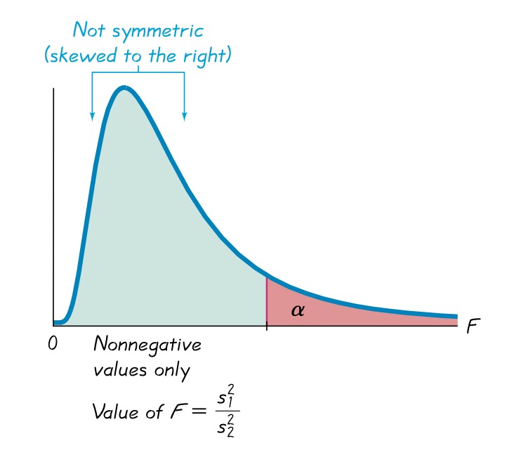
FIGURE 6.1: Two samples variance hypothesis testing reject region

Some tips for this test:

• Remember in the calculation of $F$, you need to put the larger sample variance on the numerator. In such a case, you will always get a $F$ value larger than 1. Therefore, it is not necessary to compare your $F$ value with $F_{\frac{\alpha}{2},df1,df2}$.

• To get the correct critrical value, make sure you get the correct degree of freedoms by correctly specify $n_1$ and $n_2$. You also need to judge whether this is a two-tailed test or a one-tailed test.

• F distribution table can be found as Table A-5 on your textbook or online here.

For two samples mean test, based on the result of variance test, we have two different ways.

Definition 6.3 (Test Mean of Two Samples, When Sample Variance Can Be Assumed Same) Let $\bar{x}_i,n_i,\mu_i,s_i^2$, $i=1,2$ denote the sample mean, sample size, population mean and sample variance for two groups. In this test, we usually cares about whether $\mu_1$ equals $\mu_2$ or not, the two hypotheses is then $$\begin{equation} H_0: \mu_1=\mu_2\quad\quad H_1:\mu_1\neq\mu_2 \tag{6.3} \end{equation}$$ The test statistic is then $$\begin{equation} t=\frac{\bar{x}_1-\bar{x}_2}{\sqrt{\frac{s_p^2}{n_1}+\frac{s_p^2}{n_2}}} \tag{6.4} \end{equation}$$ where $$\begin{equation} s_p^2=\frac{(n_1-1)s_1^2+(n_2-1)s_2^2}{(n_1-1)+(n_2-1)} \tag{6.5} \end{equation}$$ Since the test statistic follows t distribution under null hypothesis, the critical value should be found with respect to the t distribution table. To get the critrical value, we need to the following two values:

• Significance level $\alpha$: usually specified in the problem.

• Degree of freedom: calculated by $df=n_1+n_2-2$.

The critircal value is then $T_{\frac{\alpha}{2},df}$ and $T_{1-\frac{\alpha}{2},df}$, which give the rejection region $t<T_{\frac{\alpha}{2},df}$ or $t>T_{1-\frac{\alpha}{2},df}$. An alternative way to get conclusion is by computing the p-value. The procedure of finding p-value is summarized in Figure 6.2. We reject the null hypothesis if p-value is less than the significance level $\alpha$.

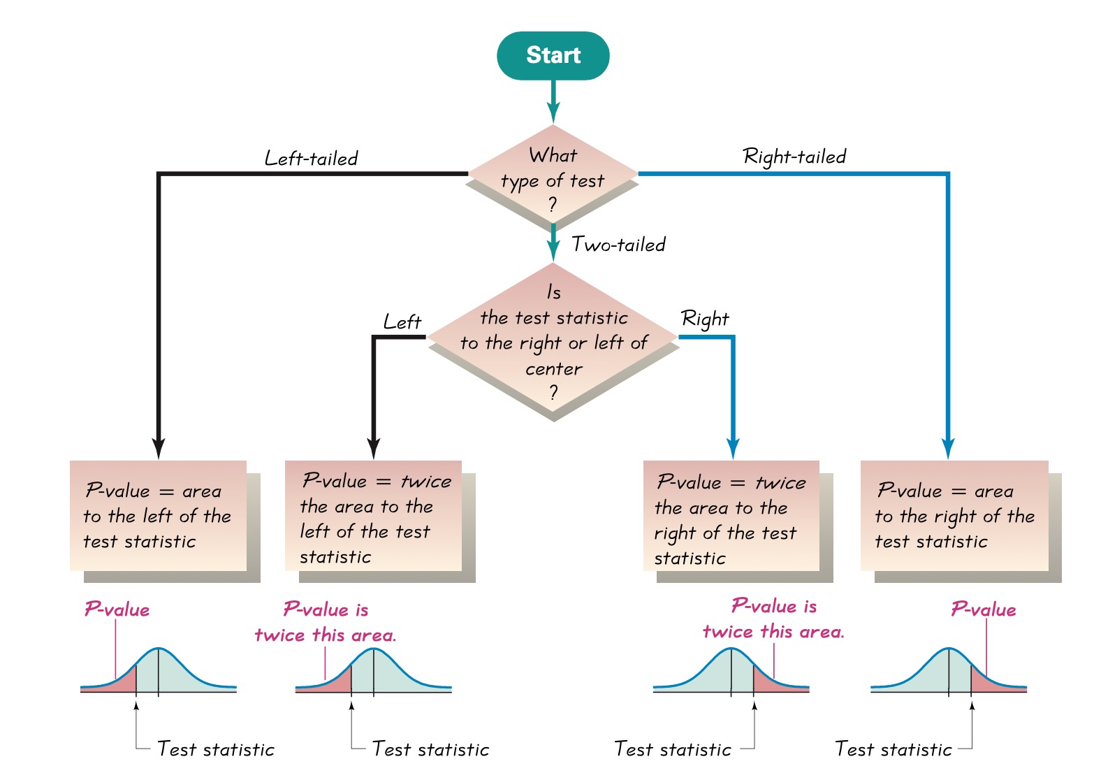
FIGURE 6.2: Procedure of finding p-value

Definition 6.4 (Test Mean of Two Samples, When Sample Variance Can NOT Be Assumed Same) Using the same notation as Definition 6.3, and the hypotheses we are going to test is still $$\begin{equation} H_0: \mu_1=\mu_2\quad\quad H_1:\mu_1\neq\mu_2 \tag{6.6} \end{equation}$$ but now the test statistic changes to $$\begin{equation} t=\frac{(\bar{x}_1-\bar{x}_2)}{\sqrt{\frac{s_1^2}{n_1}+\frac{s_2^2}{n_2}}} \tag{6.7} \end{equation}$$ To compute the critrical value, after specificing the significance level $\alpha$, you can either refer to t distribution table with $df=min\{n_1-1,n_2-1\}$ or standard normal z table. The procedure of drawing conclusion is the same as in Definition 6.3, i.e. you need to calculate p-value.

Requirements for using these tests

1. The two samples are independent.

2. Both samples are simple random samples.

3. Either or both of these conditions is satisfied: The two sample sizes are both large (with $n_1>30$ and $n_2>30$) or both samples come from populations having normal distributions.

Exercise 6.1 The test scores of randomly selected 8 female students and 6 male students are given by the following:

scores for male students: 81,84,89,79,82,90

scores for female students: 85,89,92,94,81,78,89,86.

1. Assuming the scores of females and males following $N(\mu_1,\sigma_1)$ distribution and $N(\mu_2,\sigma_2)$ distribution respectively, test the hypothesis $H_0: \sigma_1=\sigma_2$ vs. $H_1: \sigma_1\neq\sigma_2$. Would you reject $H_0$ at $5\%$ level of significance?

2. Test $H_0: \mu_1=\mu_2$ vs.$H_1:\mu_1\neq\mu_2$ and provide the p-value. Would you reject $H_0$ at 5% level of significance?

Proof. (a) We do this test step by step as the text book does.

Step 0: We compute sample variance and sample size for each groups, and denote the group with larger variance as group 1. By doing this wa have $s_1^2=29.07, n_1=8$ and $s_2^2=19.77, n_2=6$.

Step 1: The claim of equal standard deviations is equivalent to a claim of equal variances, which we express symbolically as $\sigma_1^2=\sigma_2^2$.

Step 2: If the original claim is false, then $\sigma_1^2\neq\sigma_2^2$.

Step 3: Because the null hypothesis is the statement of equality and because the alternative hypothesis cannot contain equality, we have $$\begin{equation} H_0: \sigma_1^2=\sigma_2^2\quad\quad H_1:\sigma_1^2\neq\sigma_2^2 \tag{6.8} \end{equation}$$

Step 4: The significance level is $\alpha=0.05$.

Step 5: Because this test involves two population variances, we use the F distribution.

Step 6: The test statistic is $$\begin{equation} F=\frac{s_1^2}{s_2^2}=\frac{29.07}{19.77}=1.47 \tag{6.9} \end{equation}$$ For the critrical value, we also need degree of freedom, which is 7 and 5. Thus, the critrical value is $F_{0.975,7,5}=6.85$.

Step 7: since $F=1.47<6.85$, we fail to reject the null hypothesis and conclude that the two sample standard deviation is the same.

2. We do this follows the steps given by examples on the textbook.

Step 0: The sample mean for group 1 (female students) is $\bar{x}_1=86.75$, with variance $s_1^2=29.07$ and sample size $n_1=8$. For group 2 (male students), $\bar{x}_2=84.17$, $s_2^2=19.77$ and sample size $n_2=6$.

Step 1: The claim of equal means can be expressed symbolically as $\mu_1=\mu_2$.

Step 2: If the original claim is false, then $\mu_1\neq\mu_2$.

Step 3: The alternative hypothesis is the expression not containing equality, and the null hypothesis is an expression of equality, so we have $$\begin{equation} H_0: \mu_1=\mu_2\quad\quad H_1:\mu_1\neq\mu_2 \tag{6.10} \end{equation}$$

Step 4: The significance level is $\alpha=0.05$.

Step 5: Because we have two independent samples and we are testing a claim about the two population means, we use a t distribution with the test statistic given earlier in this section.

Step 6: Since we have same variance assumption, we use Definition 6.3 to compute the test statistic as $$\begin{equation} \begin{split} &s_p^2=\frac{(n_1-1)s_1^2+(n_2-1)s_2^2}{(n_1-1)+(n_2-1)}=25.195\\ &t=\frac{\bar{x}_1-\bar{x}_2}{\sqrt{\frac{s_p^2}{n_1}+\frac{s_p^2}{n_2}}}=0.88 \end{split} \tag{6.11} \end{equation}$$

Step 7: Since the degree of freedom is $df=n+m-2=12$, we calculate p-value, the p-value for this problem as $2(1-P(t_{12}<0.88))=0.40>0.05$, so we do not reject the null hypothesis and conclude the two sample mean is the same.

There is a typo in the original solutions posted online. The sample variance in that solution is actually sample standard deviation. You need to square it so the following result all changes. The original does not follows the procedure produced on the textbook by putting the group with larger variance on the numerator. It also works but in that case you should calculate critrical value as $F_{\frac{\alpha}{2},df1,df2}$ with $df1$ and $df2$ switches.

Exercise 6.2 The heights of randomly selected 5 males from country A and 7 males from country B are given by the following:

heights for males in country A: 163,160,159,159,161

heights for males in country B: 149,182,145,143,184,185,140.

1. Assuming the heights of males from country A and B following $N(\mu_1,\sigma_1)$ distribution and $N(\mu_2,\sigma_2)$ distribution respectively, test the hypothesis $H_0: \sigma_1=\sigma_2$ vs. $H_1: \sigma_1\neq\sigma_2$. Would you reject $H_0$ at $5\%$ level of significance?

2. Test $H_0: \mu_1=\mu_2$ vs.$H_1:\mu_1\neq\mu_2$ and provide the p-value.

Proof. (a) Since $s_1^2=451.81$, $n_1=7$, $s_2^2=2.8,n_2=5$, we are testing $H_0: \sigma_1^2=\sigma_2^2$ vs. $H_1: \sigma_1^2\neq\sigma_2^2$ at significance level $\alpha=0.05$. The test statistic is $F=\frac{451.81}{2.8}=161.36$. The critrical value is $F_{0.975,6,4}=9.20$, since $F>>9.20$ we reject the null hypothesis and reject the null hypothesis, concluding that $\sigma_1\neq\sigma_2$.

For part(b) Since $\bar{x}_1=161.14$ and $\bar{x}_2=160.4$, we are testing $H_0: \bar{x}_1=\bar{x}_2$ vs. $H_1: \bar{x}_1\neq\bar{x}_2$ at significance level $\alpha=0.05$, without assuming same variance. The test statistic is therefore $$\begin{equation} t=\frac{(\bar{x}_1-\bar{x}_2)}{\sqrt{\frac{s_1^2}{n_1}+\frac{s_2^2}{n_2}}}=\frac{161.14-160.4}{\sqrt{\frac{451.81}{7}}+\sqrt{2.8}{5}}=0.09 \tag{6.12} \end{equation}$$ Then you can either compute p-value as $2(1-P(Z<0.09))=0.93$ or $2(1-P(T_4<0.09))=0.93$, either way you will fail to reject the null hypothesis and conclude the two means are the same.

Testing two proportion

This kind of hypothesis testing problem is discussed in detail in Chapter 8-2 on your textbook (start from Page-379).

Definition 6.5 (Hypothesis Testing for Two Proportions) Let $p_i,n_i,x_i,\hat{p}_i$, $i=1,2$ denote the population proportion, sample size, sample number of success, sample proportion for group 1 and 2, respectively. we have $\hat{p}_i=\frac{x_i}{n_i}$. Define $$\begin{equation} \bar{p}=\frac{x_1+x_2}{n_1+n_2} \tag{6.13} \end{equation}$$ and $\bar{q}=1-\bar{p}$. To test the hypotheses $H_0: p_1=p_2$ vs $H_1:p_0\neq p_1$ we use the test statistic $$\begin{equation} z=\frac{\hat{p}_1-\hat{p}_2}{\sqrt{\frac{\bar{p}\bar{q}}{n_1}+\frac{\bar{p}\bar{q}}{n_2}}} \tag{6.14} \end{equation}$$ This test statistic is refrred to a standard normal distribution under null hypothesis to make conclusion. The rejection region is $(-\infty,Z_{\frac{\alpha}{2}})\cup(Z_{1-\frac{\alpha}{2}},\infty)$ or we can use p-value to make conclusion. The null hypothesis is reject if the p-value is less than $\alpha$.

Exercise 6.3 A survey is conducted in the Santa Cruz and Monterey counties to assess the proportion of smokers. Among 600 people surveyed in both counties, 230 and 180 are found to be smokers in the Santa Cruz and Monterey counties respectively.

If $p_1$ and $p_2$ denote the proportion of smokers in the entire SC and Monterey counties respectively, test $H_0: p_1=p_2$ vs $H_1:p_0\neq p_1$ under $\alpha=0.05$.

Proof. We do this step by step as the textbook.

Step 0: Get the numbers from sample data, we have $n_1=n_2=600$, $x_1=230$, $x_2=180$, $\hat{p}_1=\frac{230}{600}=0.38$ and $\hat{p}_2=\frac{180}{600}=0.3$.

Step 1: The claim of equal proportion can be expressed symbolically as $p_1=p_2$.

Step 2: If the original claim is false, then $p_1\neq p_2$.

Step 3: The alternative hypothesis is the expression not containing equality, and the null hypothesis is an expression of equality, so we have $$\begin{equation} H_0: p_1=p_2\quad\quad H_1: p_1\neq p_2 \tag{6.15} \end{equation}$$

Step 4: The significance level is $\alpha=0.05$.

Step 5: The reference distribution is standard normal distribution.

Step 6: We calculate test statistic using (6.13) and (6.14) as follow. $$\begin{equation} \begin{split} &\bar{p}=\frac{x_1+x_2}{n_1+n_2}=\frac{230+180}{600+600}=0.34\\ &z=\frac{\hat{p}_1-\hat{p}_2}{\sqrt{\frac{\bar{p}\bar{q}}{n_1}+\frac{\bar{p}\bar{q}}{n_2}}}=\frac{0.38-0.3}{\sqrt{\frac{0.34\times 0.66}{600}+\frac{0.34\times 0.66}{600}}}=2.93 \end{split} \tag{6.16} \end{equation}$$

Step 7: Either compute the reject region as $(-\infty,Z_{\frac{\alpha}{2}})\cup(Z_{1-\frac{\alpha}{2}},\infty)=(-\infty,-1.96)\cup(1.96,\infty)$, $z$ is in the rejection region or compute the p-value as $2(1-P(Z<2.93))=0.003<0.05$. Either method we reject the null hypothesis and conclude that two population proportion is not the same.

Testing of Correlation This kind of hypothesis testing problem is discussed in detail in Chapter 9-2 on your textbook (start from Page-437).

Definition 6.6 (Test of Correlation) Let $n$ denote the number of pairs of data present, $r$ represents the linear correlation coefficient for a sample and $\rho$ represents the linear correlation coefficient for a population. The formula for calculate $r$ is $$\begin{equation} r=\frac{n\sum XY-(\sum X)(\sum Y)}{\sqrt{n(\sum X^2)-(sum X)^2}\sqrt{n(\sum Y^2)-(sum Y)^2}} \tag{6.17} \end{equation}$$ we are testing hypotheses $H_0:\rho=0$ vs $H_1:\rho\neq 0$. The test statistic we are using is $$\begin{equation} t=\frac{r}{\sqrt{\frac{1-r^2}{n-2}}} \tag{6.18} \end{equation}$$ Under the null hypothesis, this statistic is referred to a t distribution with $df=n-2$. You can either compute reject region defined by $(-\infty,T_{\frac{\alpha}{2},df})\cup(T_{1-\frac{\alpha}{2},df},\infty)$ or use p-value to draw conclusion.

Exercise 6.4 Theories have been developed about the heights of winning candidates for the U.S. presidency and the heights of candidates who were runners-up. Listed below are heights (in inches) from a few presidential elections.

Heights of winner: 69.5, 73, 73, 74, 74.5, 74.5, 71, 71

Heights of runners-up: 72, 69.5, 70, 68, 74, 74, 73, 76.

1. What is the correlation between the heights of winning and losing candidates?

2. Provide p-value for the test $H_0:\rho=0$ vs $H_1:\rho\neq 0$ where $\rho$ presents the unknown population correlation of heights of the winners and runners-up.

Proof. (a) Plug-in the formula (6.17) we have $r=-0.22$.

2. Since we have n=8, using (6.18) we have $t=\frac{-0.22}{\sqrt{\frac{1-(-0.22)^2}{8-2}}}=-0.55$. Hence, the p-value is $2P(T_6<-0.55)=0.60$.

In your quiz or exam, you can use a simpler way to do the problem by calculate test statistic, reject region or p-value and then make conclusion, ignoring the steps. However, if you are not confident with your answer, please follow those steps, even though you need to write a lot more, you will get more credit if you make some mistake in calculation.