Chapter 6 Numerical Solutions: Euler’s Method for Approximating Solutions of ODEs
The idea of approximating solutions to differential equations flows naturally from the graphical analysis discussed earlier. The direction field for an ODE provides a visual tool for seeing the flow of the solutions. Here we concretely approximate those solutions by using the definition of a derivative.
The simplest method for approximating solutions to initial value problems is called Euler’s method. We begin by considering an IVP:
\(y^{'} = f(t,y)\) with \(y\left( t_{0} \right) = y_{0}\) and \(t \in \left\lbrack t_{0},\ b \right\rbrack\)
In words, we have the differential equation \(y^{'} = f(t,y)\) with the
initial condition at \(t = t_{0}\) such that the solution at \(t_{0}\) is
given by: \(y\left( t_{0} \right) = y_{0}\). We are interested in \(t\)
values in the interval \(t_{0} \leq t \leq b\).
Note: for a numerical approximation we need a finite interval, so \(t\)
must have an ending value, \(b\).
For this IVP, we may have a known analytical solution, \(y(t)\), or we may need to approximate the solution using the information given to us. As with all first order ODEs, we can calculate how quickly the solution is changing, \(y'\), if we know the current time and the current value of the solution.
6.1 Euler’s Method
Consider the definition of the derivative for the function \(y(t)\):
\[\frac{dy}{dt}(t) = y^{'}(t) = \lim_{\Delta t \rightarrow 0}\left( \frac{y(t + \Delta t) - y(t)}{\Delta t} \right)\]
For any numerical method, we must choose a value for \(\Delta t\) which means \(\Delta t \rightarrow 0\) is not possible. Once we have selected a value for \(\Delta t\), we can approximate the derivative. Notice that the smaller we choose \(\Delta t\), the better our approximation for the derivative. For a fixed \(\Delta t\) value we have:
\[y^{'}(t) \approx \frac{y(t + \Delta t) - y(t)}{\Delta t}\]
This is the foundation for Euler’s method. Solving the approximation for \(y(t + \Delta t)\) gives
\[\Delta t\cdot y^{'}(t) \approx y(t + \Delta t) - y(t)\]
\[y(t + \Delta t) \approx y(t) + \Delta t\cdot y^{'}(t)\] This formula tells us how to approximate \(y(t+\Delta t)\), that is, the value of \(y\) at a later time, if we know the current value of \(y\) and the current value of the derivative of \(y\), \(y'\). Crucially, the ODE tells us how to calculate \(y'\).
Inherent within Euler’s method is the fact that the function’s domain, i.e. the \(t\) interval, has been segmented into a fixed set of equally spaced points, based on \(\Delta t\).
Recall from the definition of the initial value problem that the domain of interest is \(t \in \left\lbrack t_{0},b \right\rbrack\). The end point of the interval is required for computation.

Now a step size, \(\Delta t\), is selected. As a result of choosing \(\Delta t\), we have a finite number of values where we will estimate the function.

We number these values starting at \(t_{0}\), which is given with the initial condition, and continue as \(t_{1}\), \(t_{2}\), \(t_{3}\), … until the endpoint, \(t_{N} = b\), is reached. In general, we have \(N\) subintervals of length \(\Delta t\). The number \(N\) is determined by the length of \(\Delta t\). In fact these two quantities are related via
\[\Delta t = \frac{b - t_{0}}{N}\]
The set of domain values where we will approximate \(y(t)\) is given as:
\[t_{n} = t_{0} + n\Delta t\ \ \ for\ \ \ n = 0,1,\ldots,N\]
Through this set of \(t_{n}\) values, we rewrite Euler’s method from the
approximation
\[\begin{aligned}
&{y(t + \Delta t) \approx y(t) + \Delta t\cdot y^{'}(t)
}\\
&{y\left( t_{n} + \Delta t \right) \approx y\left( t_{n} \right) + \Delta t \cdot y^{'}\left( t_{n} \right)
}\\
&{y\left( t_{n + 1} \right)
\approx y\left( t_{n} \right) + \Delta t\cdot y^{'}\left( t_{n} \right)}\end{aligned}\]
since \(t_{n + 1} = t_{n} + \Delta t\). We now see the recursive nature of this calculation. The table below shows the initial condition, \(\left( t_{0},y_{0} \right)\), in the blue circles. Euler’s method is worked from left to right by calculating the slope, \(y'(t_{n})\), and the next approximation \(y\left( t_{n + 1} \right)\). Note: the step size \(\Delta t\) is fixed for the entire computation, and the following notation is used: \(y_{n} \equiv y\left( t_{n} \right)\).

The next Euler calculation is based on the output from the previous step – this is recursion. In fact this tabular format provides an excellent tool for setting up and executing Euler approximations, and several exercises will use this approach. When several thousands or millions of calculations are required, we program Euler’s method into a computer.
6.1.1 Example
Approximate the solution for this IVP: \[y^{'} = \sin(t) \text{ with } y(0) = 1 \text{ and } t \in \lbrack 0,\ 6\rbrack\]
We start by selecting a step size for the calculation. Let
\(\Delta t = 0.25\). This is a choice that we’ll have to make. Smaller \(\Delta t\) will yield more accurate results, but requires more calculations on our part. Next, we understand the values in the domain where we
will approximate the function: \(t_{0} = 0\), \(t_{1} = 0.25\),
\(t_{2} = 0.5\), …. For this example we have \(t_{n} = 0.25n\). Finally,
we apply Euler’s method using the initial function value: \(y(0) = 1\).
Here is Euler’s method for this specific IVP
\[y\left( t_{n + 1} \right) \approx y\left( t_{n} \right) + \Delta t y'(t_n).\]
Now, the ODE tells us how to compute \(y'(t_n)\). It says that \(y'(t_n)=\sin(t_n)\), we we’ll be computing
\[y(t_{n+1})=y(t_n)+\Delta t \sin(t_n).\]
Since we’ve chosen \(\Delta t = 0.25\) we finally get
\[y(t_{n+1})=y(t_n)+0.25\sin(t_n).\]
Note: we often use the shorthand \(y_{n} \equiv y\left( t_{n} \right)\)
which gives a slightly different appearance
\[y_{n + 1} \approx y_{n} + 0.25\sin\left( t_{n} \right)
\]Setting up a table helps to keep Euler’s method organized, and the
numerical approximation is provided in the table below.
For this problem, we can also solve the IVP analytically.
\(y^{'} = \sin(t)\) with \(y(0) = 1\) and \(t \in \lbrack 0,\ 6\rbrack\)
Recall:
\[\int_{}^{}{y^{'}(t)dt} = \int_{}^{}{\sin(t)dt}\]
\[y(t) = - \cos(t) + C
\]With the general solution, we apply the IC giving
\[y(0) = 1 = - 1 + C\]
\[C = 2\]
The specific solution is
\[y(t) = - \cos(t) + 2.\]
The table showing the Euler’s method approximation for \(y^{'} = \sin(t)\) with \(y(0) = 1\) and \(t \in \lbrack 0,\ 6\rbrack\)

We can use the analytical solution to check the accuracy of Euler’s method. Note that the reason we would use Euler’s method is because we usually can’t find an analytical solution. Using the analytical solution to check the accuracy of Euler’s method is fairly artificial, since if we can find an analytical solution we won’t bother with approximation via Euler’s method. Nevertheless, in this case, we can calculate how much error Euler’s method produced. The error in Euler’s method at timestep \(n\) is defined to be \(|y_n-y(t_n)|\). That is, it is the absolute value of the difference between the analytical solution at time \(t_n\) and the Euler approximation at time \(t_n\). Below is a table calculating the error in our Euler’s method approximation to \(y\) at each time step.
| \(n\) | \(t_n\) | \(y_n\) | \(y(t_n)\) | error=\(abs(y(t_n)-y_n)\) |
|---|---|---|---|---|
| 1 | 0.00 | 1.000000 | 1.000000 | 0.0000000 |
| 2 | 0.25 | 1.000000 | 1.031088 | 0.0310876 |
| 3 | 0.50 | 1.061851 | 1.122417 | 0.0605664 |
| 4 | 0.75 | 1.181707 | 1.268311 | 0.0866038 |
| 5 | 1.00 | 1.352117 | 1.459698 | 0.1075806 |
| 6 | 1.25 | 1.562485 | 1.684678 | 0.1221928 |
| 7 | 1.50 | 1.799731 | 1.929263 | 0.1295318 |
| 8 | 1.75 | 2.049105 | 2.178246 | 0.1291413 |
| 9 | 2.00 | 2.295101 | 2.416147 | 0.1210456 |
| 10 | 2.25 | 2.522426 | 2.628174 | 0.1057481 |
| 11 | 2.50 | 2.716944 | 2.801144 | 0.0841998 |
| 12 | 2.75 | 2.866562 | 2.924302 | 0.0577405 |
| 13 | 3.00 | 2.961977 | 2.989993 | 0.0280154 |
| 14 | 3.25 | 2.997257 | 2.994130 | 0.0031275 |
| 15 | 3.50 | 2.970208 | 2.936457 | 0.0337517 |
| 16 | 3.75 | 2.882513 | 2.820559 | 0.0619532 |
| 17 | 4.00 | 2.739622 | 2.653644 | 0.0859786 |
| 18 | 4.25 | 2.550422 | 2.446087 | 0.1043341 |
| 19 | 4.50 | 2.326674 | 2.210796 | 0.1158785 |
| 20 | 4.75 | 2.082292 | 1.962398 | 0.1198939 |
| 21 | 5.00 | 1.832469 | 1.716338 | 0.1161307 |
| 22 | 5.25 | 1.592737 | 1.487915 | 0.1048229 |
| 23 | 5.50 | 1.378004 | 1.291330 | 0.0866736 |
| 24 | 5.75 | 1.201619 | 1.138808 | 0.0628112 |
| 25 | 6.00 | 1.074549 | 1.039830 | 0.0347193 |
6.2 Euler’s Method and Direction Fields
To fully understand Euler’s method, we will relate it to the graphical analysis we discussed earlier. The two ideas are closely linked. For both the direction fields and Euler’s method, we are using the one thing we know for certain … the rate of change! This information is available in every first order ODE.
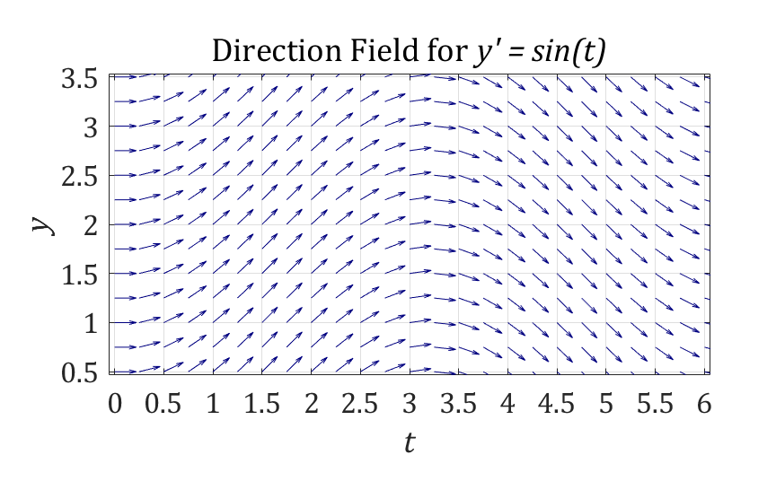
Returning to our example, the direction field for the differential equation
\[y^{'} = \sin(t)\]
is shown above.
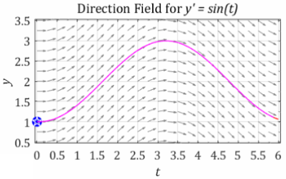
Given the initial condition \(y(0) = 1\), we consider the flow of a ball along the “river” created by the direction field. Our approximation of this flow can be seen here. This is exactly the same as we discussed in Section 3. The question is this: how did we approximate the flow of the solution along the direction field?
The answer: Euler’s Method
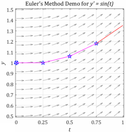
The picture above shows the connection between a direction field and Euler’s method. The graphic follows the previous example with the IVP:
\(y^{'} = \sin(t)\) with \(y(0) = 1\) and \(t \in \lbrack 0,\ 6\rbrack\)
and step size set to \(\Delta t = 0.25\). The graphic is zoomed in to consider only \(0 \leq t \leq 1\).
We look closely at Euler’s method:
\[y\left( t_{n + 1} \right) = y\left( t_{n} \right) + \Delta t\cdot y^{'}\left( t_{n} \right)\]
and focus on the term \(\Delta t\cdot y^{'}\left( t_{n} \right)\). The rate of change, \(y^{'}\left( t_{n} \right)\), is represented as the slope of the red line at each time step. The slope projects forward, and the change in the function value is given by \(\Delta t\cdot y^{'}\left( t_{n} \right)\). This change is added to the previous function value, \(y\left( t_{n} \right)\).

As a result, the new value, \(y\left( t_{n + 1} \right)\), is shown by the height at the end of the red line. The actual end of the red line is the next value of the approximated solution graph: \(\left( t_{n + 1},y\left( t_{n + 1} \right) \right)\). The process is repeated as Euler’s method moves to the next time step. Note: the blue stars are the approximated points, \(\left( t_{n + 1},y\left( t_{n + 1} \right) \right)\), and these points match the points in the table shown with the example problem. From the graphic we can clearly see why smaller step sizes give more accurate approximations.
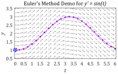
The complete approximation with \(\Delta t = 0.25\) is shown above. Again, the blue stars are the points that have actually been calculated using Euler’s method. All of the previous solutions shown with direction fields have been calculated in this way. The picture at the beginning of this example uses a much smaller value of \(\Delta t = 0.125\) and omits the blue stars.
6.3 Examples Using Euler’s Method
6.3.1 Example 2
Use Euler’s method to approximate the solution for this IVP. Use \(\Delta t = 0.25\) .
\[y^{'} = (y-1)t\ \ \text{ with}\ \ \ y(0) = - 1\ \ \text{ and}\ \ \ t \in \lbrack 0,1\rbrack.\] To begin, we know from the initial condition that \(y(0)=-1\). Remember that \(y_0\) is our approximation to the value of \(y\) at the 0\(^{th}\) time step, which in this case is at time \(t_0=0\). So we’ll set \[y_0=y(0)=-1.\] Next, we’ll calculate \(y_1\). Because we’ve chosen our time step to be \(\Delta t=0.25\), \(y_1\) will be our approximation to the value of \(y\) at time \(t_1=0+0.25=0.25\). The formula for using Euler’s method says: \[y(0.25)\approx y_1 = y_0 + \Delta t y'(t_0).\] We already have the value of \(y_0=-1\), and we can use the ODE to calculate the value of \(y'(t_0)\). \[\begin{aligned} y'(t_0) &= (y_0-1)t_0 =(-1-1)\cdot 0\\ &=0.\end{aligned}\] Plugging this value into our formula for Euler’s method gives us \[y(0.25)\approx y_1 = y_0 + \Delta t \cdot 0 = -1 + 0.25 \cdot 0 =-1.\] So, we estimate that the value of \(y\) at time \(t_1=0.25\) is also \(-1\). Now we can calculate \(y_2\). Again, because our step size is \(\Delta t=0.25\), \(y_2\) is our approximation to the value of \(y\) at time \(t_2=t_1 + 0.25 =0.5\).
The formula for Euler’s method tells us: \[y(0.5)\approx y_2 = y_1 + \Delta t y'(t_1).\] We can use the ODE to calculate \(y'(t_1)\). \[y'(t_1)= (y_1 -1)t_1 = (-1 -1)0.25 = -0.5.\] Now we use this value of \(y'(t_1)\) in our formula to get \[y(0.5)\approx y_2 = y_1 + \Delta t y'(t_1) = -1 + 0.25\cdot -0.5 = -1.125.\] Next we compute \(y_3\), which is our approximation to the value of \(y\) at time \(t_3=t_2+0.25=0.75\). Euler’s method tells us to calculate \[y(t_3)\approx y_3 = y_2 +\Delta t y'(t_2).\] To compute \(y'(t_2)\) we use the ODE. \[y'(t_2)=(y_2-1)t_2=-1.0625.\]
Inserting this into our Euler’s method formula gives \[y(t_3)\approx y_3 = y_2 +\Delta t y'(t_2)= -1.125 + 0.25\cdot -1.0625 = -1.390625.\] Finally, we are ready to compute \(y_4\), which will be our approximation to the value of \(y\) at time \(t_4=t_3+0.25=1\), and 1 is the end of the time interval we are interested in. The method says that \[y(1)\approx y_4=y_3+\Delta t y'(t_3).\] We can use the ODE to calculate \[y'(0.75) = (y_3 - 1)\Delta t = -1.7929688.\] Inserting this into our formula for \(y_4\) gives us \[y(1)\approx y_4=y_3+\Delta t y'(t_3) = -1.390625 + 0.25 \cdot -1.7929688 = -1.8388672.\] We are now done, having successfully approximated \(y(0.25)\), \(y(0.5)\), \(y(0.75)\), and \(y(1)\).
These computations are often easier to execute using a table, such as the one below.
| \(n\) | \(t_n\) | \(y_n\) | \(y'_n=(y_n-1)t_n\) | \(y_n+\Delta t\cdot y'_n\) |
|---|---|---|---|---|
| 0 | 0 | -1 | 0 | -1 |
| 1 | 0.25 | -1 | -0.5 | -1.125 |
| 2 | 0.5 | -1.125 | -1.0625 | -1.390625 |
| 3 | 0.75 | -1.390625 | -1.7929688 | -1.8388672 |
| 4 | 1 | -1.8388672 | - | - |
6.3.1.1 Example 3
Use Euler’s method to approximate the solution for this IVP. Use \(\Delta t = \frac{1}{2}\) .
\[y' = \cos(t)+y, \text{ with } y(2)=4 \text{ and } t\in [2,6].\] This time, the initial condition is given at time 2. So we set \(t_0=2\) and use \(y_0=4\).
Now, we proceed as in the previous example.
Since our step size is now 0.5, \(t_1=t_0+0.5=2.5\). \(y_1\) is our approximation to the value of \(y\) at time \(t_1=2.5\).
The formula for Euler’s method says that \[y(2.5)\approx y_1 = y_0 + \Delta t y'(t_0).\] To calculate \(y'(t_0)\) we use the ODE. \[y'(t_0)=\cos(t_0)+y_0 = \cos(2)+4 = 1.346.\] Inserting this into the formula for \(y_1\) gives us \[y(2.5)\approx y_1 = y_0 + \Delta t y'(t_0) = 4 + 0.5\cdot 1.346=4.673.\]
Continuing, \(t_2=t_1+0.5=3\). \(y_2\) is our approximation to the value of \(y\) at time \(t_2=3\).
The formula for Euler’s method says that \[y(3)\approx y_2 = y_1 + \Delta t y'(t_1).\] To calculate \(y'(t_1)\) we use the ODE. \[y'(t_1)=\cos(t_1)+y_1 = \cos(2.5)+4.673 = 2.461.\] Inserting this into the formula for \(y_1\) gives us \[y(3)\approx y_2 = y_1 + \Delta t y'(t_1) = 4.673 + 0.5\cdot 2.461=5.904.\]
Continuing, \(t_3=t_2+0.5=3.5\). \(y_3\) is our approximation to the value of \(y\) at time \(t_3=3.5\).
The formula for Euler’s method says that \[y(3.5)\approx y_3 = y_2 + \Delta t y'(t_2).\] To calculate \(y'(t_2)\) we use the ODE. \[y'(t_2)=\cos(t_2)+y_2 = \cos(3)+5.904 = 3.929.\] Inserting this into the formula for \(y_1\) gives us \[y(3.5)\approx y_3 = y_2 + \Delta t y'(t_2) = 5.904 + 0.5\cdot 3.929=7.868.\]
Continuing, \(t_4=t_3+0.5=4\). \(y_4\) is our approximation to the value of \(y\) at time \(t_4=4\).
The formula for Euler’s method says that \[y(4)\approx y_4 = y_3 + \Delta t y'(t_3).\] To calculate \(y'(t_3)\) we use the ODE. \[y'(t_3)=\cos(t_3)+y_3 = \cos(3.5)+7.868 = 3.486.\] Inserting this into the formula for \(y_1\) gives us \[y(4)\approx y_4 = y_3 + \Delta t y'(t_3) = 7.868 + 0.5\cdot 3.486=9.611.\]
Continuing, \(t_5=t_4+0.5=4.5\). \(y_5\) is our approximation to the value of \(y\) at time \(t_5=4.5\).
The formula for Euler’s method says that \[y(4.5)\approx y_5 = y_4 + \Delta t y'(t_4).\] To calculate \(y'(t_4)\) we use the ODE. \[y'(t_4)=\cos(t_4)+y_4 = \cos(4)+9.611 = 3.017.\] Inserting this into the formula for \(y_1\) gives us \[y(4.5)\approx y_5 = y_4 + \Delta t y'(t_4) = 9.611 + 0.5\cdot 3.017=11.12.\]
Continuing, \(t_6=t_5+0.5=5\). \(y_6\) is our approximation to the value of \(y\) at time \(t_6=5\).
The formula for Euler’s method says that \[y(5)\approx y_6 = y_5 + \Delta t y'(t_5).\] To calculate \(y'(t_5)\) we use the ODE. \[y'(t_5)=\cos(t_5)+y_5 = \cos(4.5)+11.12 = 4.624.\] Inserting this into the formula for \(y_1\) gives us \[y(5)\approx y_6 = y_5 + \Delta t y'(t_5) = 11.12 + 0.5\cdot 4.624=13.431.\]
Continuing, \(t_7=t_6+0.5=5.5\). \(y_7\) is our approximation to the value of \(y\) at time \(t_7=5.5\).
The formula for Euler’s method says that \[y(5.5)\approx y_7 = y_6 + \Delta t y'(t_6).\] To calculate \(y'(t_6)\) we use the ODE. \[y'(t_6)=\cos(t_6)+y_6 = \cos(5)+13.431 = 5.649.\] Inserting this into the formula for \(y_1\) gives us \[y(5.5)\approx y_7 = y_6 + \Delta t y'(t_6) = 13.431 + 0.5\cdot 5.649=16.256.\]
Continuing, \(t_8=t_7+0.5=6\). \(y_8\) is our approximation to the value of \(y\) at time \(t_8=6\).
The formula for Euler’s method says that \[y(6)\approx y_8 = y_7 + \Delta t y'(t_7).\] To calculate \(y'(t_7)\) we use the ODE. \[y'(t_7)=\cos(t_7)+y_7 = \cos(5.5)+16.256 = 4.646.\] Inserting this into the formula for \(y_1\) gives us \[y(6)\approx y_8 = y_7 + \Delta t y'(t_7) = 16.256 + 0.5\cdot 4.646=18.579.\]
Once again, it is easiest to organize the calculations in a table.
| \(n\) | \(t_n\) | \(y_n\) | \(y'_n=\cos(t_n)+y_n\) | \(y_n+\Delta t\cdot y'_n\) |
|---|---|---|---|---|
| 0 | 2 | 4 | 1.346 | 4.673 |
| 1 | 2.5 | 4.673 | 2.461 | 5.904 |
| 2 | 3 | 5.904 | 3.929 | 7.868 |
| 3 | 3.5 | 7.868 | 3.486 | 9.611 |
| 4 | 4 | 9.611 | 3.017 | 11.12 |
| 5 | 4.5 | 11.12 | 4.624 | 13.431 |
| 6 | 5 | 13.431 | 5.649 | 16.256 |
| 7 | 5.5 | 16.256 | 4.646 | 18.579 |
| 8 | 6 | 18.579 | - | - |
6.3.1.2 Example #4
Use Euler’s method to approximate the solution for this IVP. Use \(\Delta t = 0.125\) .
\[y^{'} = 1 - y + \ln(t) \text{ with } y(1) = 0 \text{ and }t \in \lbrack 1,\ 3\rbrack\]
By now we are convinced that organizing our calculations in a table is the way to go. The table is shown below.
| \(n\) | \(t_n\) | \(y_n\) | \(y'_n=1-y_n+\ln(t_n)\) | \(y_n+\Delta t\cdot y'_n\) |
|---|---|---|---|---|
| 0 | 1 | 0 | 1 | 0.125 |
| 1 | 1.125 | 0.125 | 0.993 | 0.249 |
| 2 | 1.25 | 0.249 | 0.974 | 0.371 |
| 3 | 1.375 | 0.371 | 0.947 | 0.489 |
| 4 | 1.5 | 0.489 | 0.916 | 0.604 |
| 5 | 1.625 | 0.604 | 0.882 | 0.714 |
| 6 | 1.75 | 0.714 | 0.846 | 0.82 |
| 7 | 1.875 | 0.82 | 0.809 | 0.921 |
| 8 | 2 | 0.921 | 0.772 | 1.017 |
| 9 | 2.125 | 1.017 | 0.737 | 1.109 |
| 10 | 2.25 | 1.109 | 0.702 | 1.197 |
| 11 | 2.375 | 1.197 | 0.668 | 1.281 |
| 12 | 2.5 | 1.281 | 0.635 | 1.36 |
| 13 | 2.625 | 1.36 | 0.605 | 1.436 |
| 14 | 2.75 | 1.436 | 0.576 | 1.508 |
| 15 | 2.875 | 1.508 | 0.548 | 1.576 |
| 16 | 3 | 1.576 | - | - |
6.4 Using R to Perform Euler’s Method
Using Euler’s method to compute an approximate solution to an ODE is not hard. It is, however, quite tedious and prone to arithmetic mistakes. This makes it perfect for R to do for us. The command Euler performs Euler’s method for us.
As with plotODEDirectionField, we need only specify the right hand side of our ODE. We’ll also need to specify the initial condition for the problem, the step size (\(\Delta t\)), and the time over which to approximate the solution. To approximate a solution to
\[y'=(y-1)t,\,y(0)=-1,\,t\in[0,1]\]
with step size \(\Delta t = 0.25\), we issue the following command. It is important to list the variables in the order \(t\), \(y\), when using any command related to differential equations.
##      t         y
## 1 0.00 -1.000000
## 2 0.25 -1.000000
## 3 0.50 -1.125000
## 4 0.75 -1.390625
## 5 1.00 -1.838867
This matches with our results above.
To approximate a solution to the IVP \[y^{'} = 1 - y + \ln(t) \text{ with } y(1) = 0 \text{ and }t \in \lbrack 1,\ 3\rbrack\] using step size \(\Delta t = 0.125\), we issue the following command.
##        t         y
## 1  1.000 0.0000000
## 2  1.125 0.1250000
## 3  1.250 0.2490979
## 4  1.375 0.3708536
## 5  1.500 0.4893036
## 6  1.625 0.6038238
## 7  1.750 0.7140343
## 8  1.875 0.8197320
## 9  2.000 0.9208416
## 10 2.125 1.0173798
## 11 2.250 1.1094288
## 12 2.375 1.1971165
## 13 2.500 1.2806016
## 14 2.625 1.3600627
## 15 2.750 1.4356900
## 16 2.875 1.5076789
## 17 3.000 1.5762256
6.5 Exercises
For each IVP, create a table to compute the first three iterations of Euler’s method by hand (use a calculator or R to do the arithmetic). Create
and label the columns exactly as we have done throughout this section:
\(n\), \(t_n\), \(y_n\), \(y^{'}_n\), and \(y_n + \Delta t\cdot y^{'}_n\). Once you are done, use Euler to compute the entire table, and check your work.
\(y^{'} = \cos\left( t - \sqrt{t} \right)\) with \(y(0) = - 4\) and \(t \in \lbrack 0,\ 10\rbrack\). Use \(\Delta t = \frac{1}{2}\)
\(y^{'} = (1 - y)^{2}\) with \(y(0) = - 1\) and \(t \in \lbrack 0,\ 15\rbrack\). Use \(\Delta t = \frac{1}{4}\)
\(y^{'} = e^{-t+y}\) with \(y(1) = 0\) and \(t \in \lbrack 1,\ 6\rbrack\). Use \(\Delta t = \frac{1}{16}\)
\(y^{'} = t - |y|\) with \(y(0) = 2\) and \(t \in \lbrack 0,\ 12\rbrack\). Use \(\Delta t = \frac{1}{4}\)