Chapter 9 Modeling: Equilibrium Solutions and Stability

In Section 5.2 we noted that autonomous ODEs have very simple direction fields, since the slopes to not vary in the $t$-direction.
Since each column of vectors is identical in the direction field, we can condense the information from the direction field. We need only consider the rates of change at a single value of $t$. This leads to the phase line plot which shows directions in which solutions flow.

Because the phase line summarizes all of the information in the direction field for an autonomous ODE, we frequently only present the phase line.

The phase line plot also includes the equilibrium solutions, and it provides a quick way to visually represent the flow of solutions for autonomous, 1^st order ODEs.

9.1 Equilibrium Solutions

The simplest solution to a differential equation is a solution that remains constant for all time. Such solutions are called equilibrium solutions.

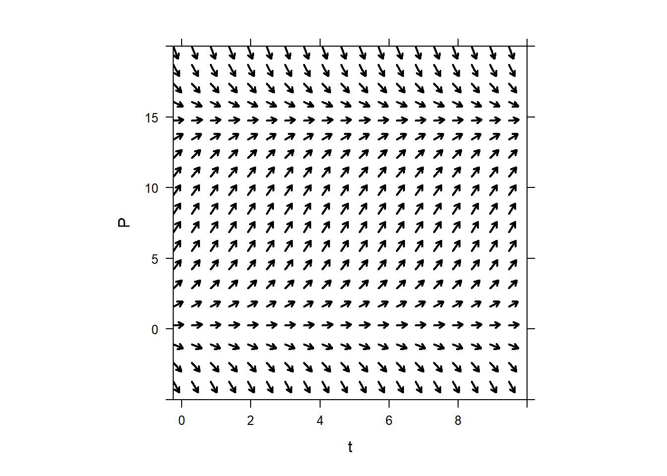
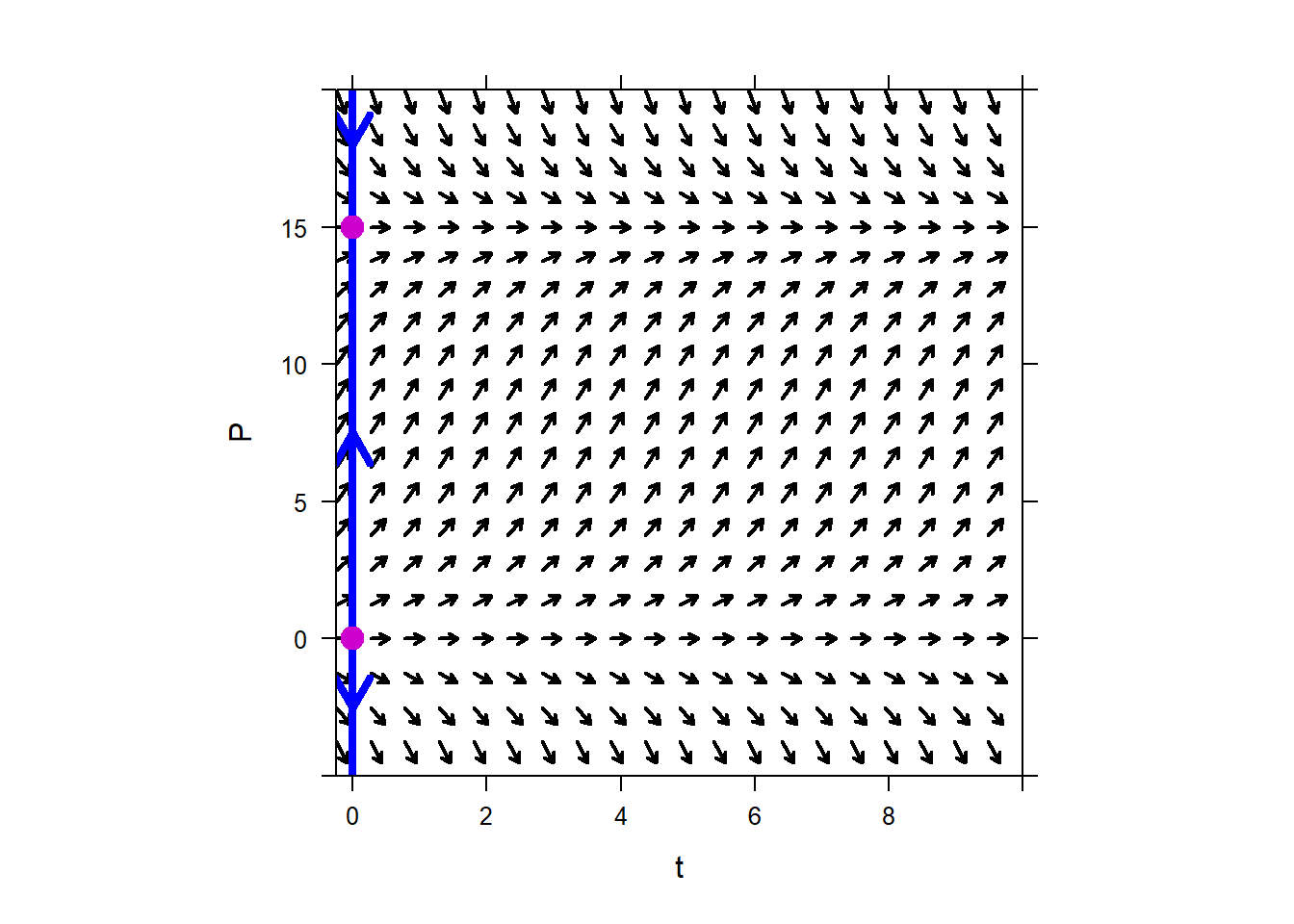
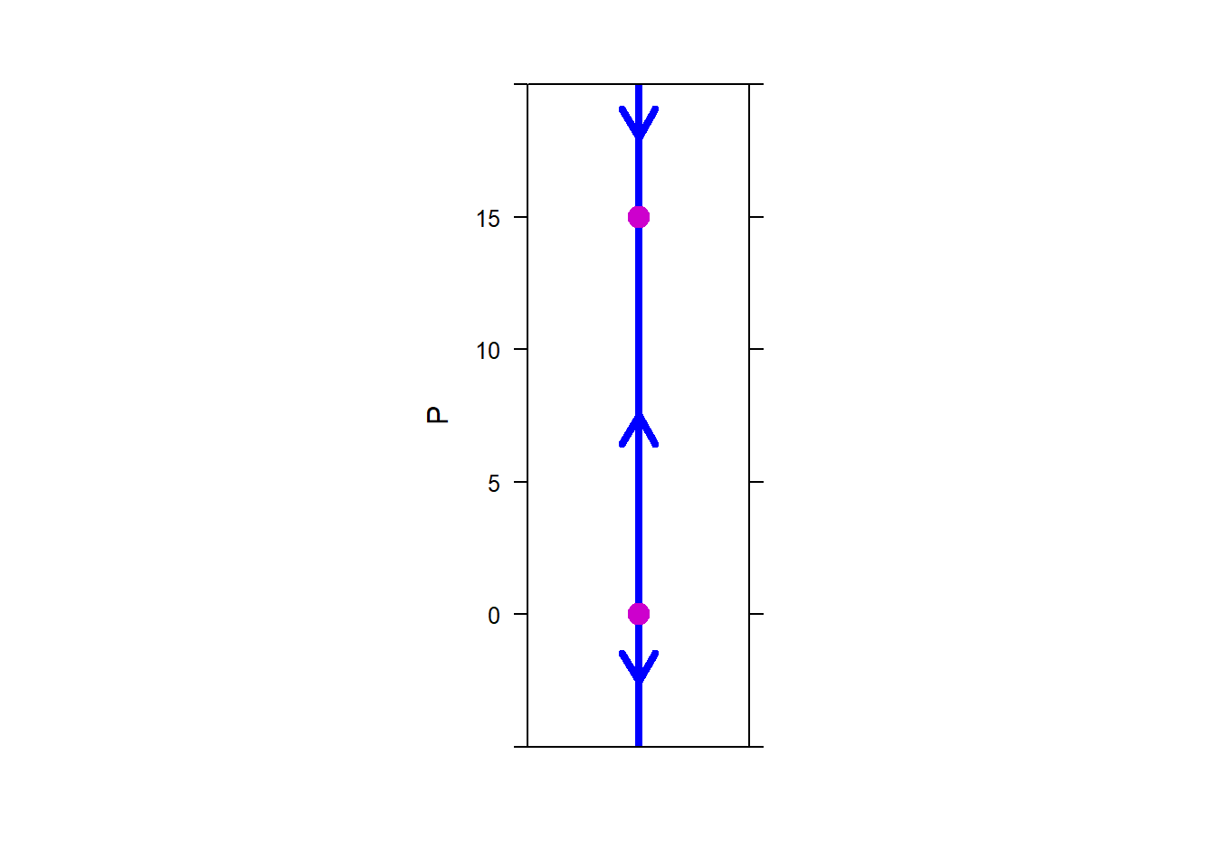
Equilibrium solutions to a given ODE are solutions to the ODE that are constant. Suppose that $y$ is an equilibrium solution to $$y'=f(y).$$ Because $y$ is an equilibrium solution, it is constant. Because it is constant, it must have zero derivative, $y'=0$. Because it satisfies the ODE, $y'=f(y)$. So, we can find equilibrium solutions by finding all constant values of $y$ that satisfy $$f(y)=0.$$ For example, consider a population of squirrels whose population is modeled by $$P'=0.3P\left(1-\frac{P}{15}\right).$$ In order to find equilibrium solutions, we solve $$0=0.3P\left(1-\frac{P}{15}\right)$$ for $P$. The equilibrium solutions are $$P=0,\text{ and }P=15.$$ We can interpret equilibrium solutions as saying “If the population of squirrels starts at 0 or 15, the population of rabbits will never change”.

Equilibrium solutions are key components of autonomous differential equations. A solution to a 1^st order, autonomous ODE always does one of three things:

• The solution is an equilibrium solution.

• The solution approaches an equilibrium solution.

• The solution approaches positive or negative infinity.

The prominence of equilibrium solutions leads to the importance of the phase line plot. While the phase line plot does not provide the specific rates of change for solutions, it does provide the direction of change. The phase line shows us when a solution is an equilibrium solution, is approaching (or leaving) an equilibrium solution, or is approaching $\pm \infty$.

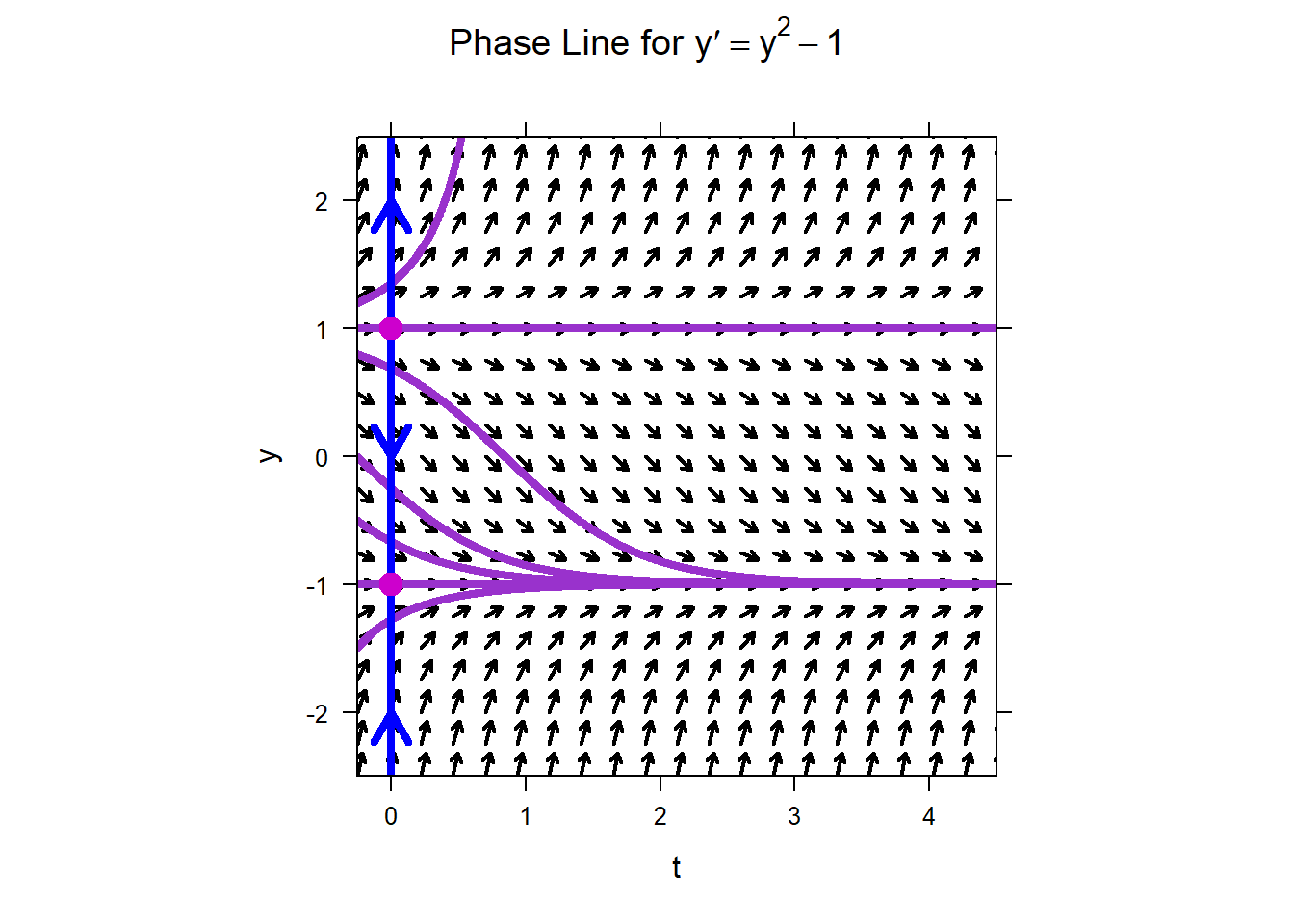
The plot on the right shows several solutions with different initial conditions. Notice the correlation between the solutions and the phase line plot.

For the given ODE

$$y^{'} = y^{2} - 1\ ,$$

the solutions $y(t) = 1$ and $y(t) = - 1$ are equilibrium solutions. They are constant for all values of $t$. Solutions with initial conditions between $- 1$ and 1, i.e. $y_{0} \in ( - 1,1)$, approach the equilibrium solution $y(t) = - 1$ as $t$ increases. Similarly, initial conditions less than $- 1$ generate solutions that also approach this equilibrium solution. By contrast, initial conditions greater than 1 generate solutions that approach $+$infinity as $t$ increases. All of this information is captured by the phase line.

9.2 Stability

An equilibrium solution, $y^{*}$, is stable if any solution $y(t)$ with an initial condition "near" $y^{*}$ stays near the equilibrium solution for all time. In the case of a single ODE, an equilibrium solution is stable if all solutions with initial conditions near the equilibrium solution tend toward the equilibrium solution. However, when we deal with systems, we will see that actually an equilibrium solution is stable if nearby initial conditions lead to solutions that “don’t run away” from the equilibrium solution. The concept of “nearby initial conditions” is not rigorously defined.

An equilibrium solution, $y^{*}$, is unstable if solutions starting "near" $y^{*}$ move away from $y^{*}$ as $t$ approaches infinity.

For example, the equilibrium solutions for $$y^{'} = y^{2} - 1$$ are $y=1$ and $y=-1$. By looking at the phase portraits, we can see that any initial condition “near” the equilibrium solution -1 leads to a solution to ODE that tends toward the equilibrium solution.

Therefore, $y=-1$ is a stable equilibrium solution. On the other hand, initial conditions near 1 lead to solutions that diverge away from the equilibrium solution $y=1$. Therefore, we say that $y=1$ is an unstable equilibrium solution.

In fact, the solution continues to decrease as long as the value $y$ is larger than $- 1$. The flow of this solution is provided by the phase line and is easy to visualize with the direction field. It is true that though the solutions will approach the equilibrium solutions, they will never quite reach them. This fact will be studied thoroughly in a class on ODEs.

We can build a phase line by hand by 1) finding the equilibrium solutions by hand, using algebra, 2) determining whether solutions to the ODE increase or decrease by testing their derivative using the ODE, similar to the first derivative test.

9.2.1 Example 1

Find the equilibrium solutions and plot the phase line for $$y^{'} = y\left( 4 - y^{2} \right)$$

To find the equilibrium solutions we solve $y^{'} = 0$:

$$y\left( 4 - y^{2} \right) = 0$$

$$y(2 - y)(2 + y) = 0$$

The equilibrium solutions for this ODE are $y = 0$, $y = 2$, and $y = - 2$. To find the directions in which the solutions flow, we determine the rates of change between the equilibrium solutions. In this case we will check the rates when $y = - 3, - 1,\ 1,\ 3$.

For instance, suppose a solution starts at an initial condition below -2, for instance -3. Then the solution moves with derivative $$y'=-3\cdot(2-(-3)(2+(-3))=15>0.$$ Therefore, the solution is increasing if it starts out at -3. In fact, the solution will be increasing if it starts out anywhere below -2. We can repeat this test for solutions between -2 and 0, between 0 and 2, and larger than 2 similaraly, and summarize the results in a table, as below.

$y$	$y'$	Interpretation
$- 3$	$( - 3)\left( 4 - ( - 3)^{2} \right) = 15$	Solutions less than $-2$ are increasing
$- 1$	$( - 1)\left( 4 - ( - 1)^{2} \right) = - 3$	Solutions between $-2$ and $0$ are decreasing
$1$	$(1)\left( 4 - 1^{2} \right) = 3$	Solutions between $0$ and $2$ are increasing
$3$	$(3)\left( 4 - 3^{2} \right) = - 15$	Solutions larger than $2$ are decreasing

With this information, we can draw the phase line. 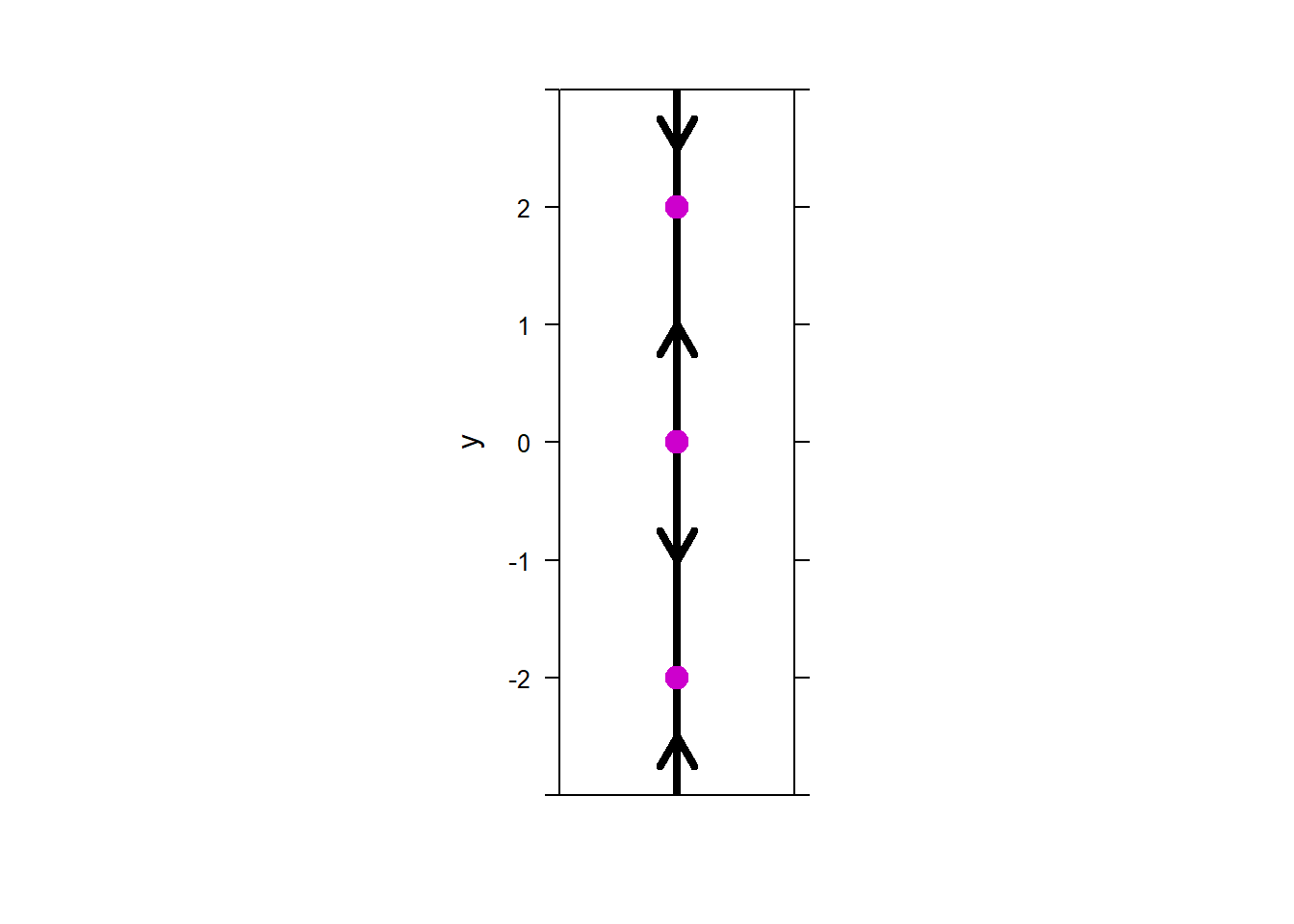The phase line plot shows us that the equilibrium solutions have the following stability:

• $y = - 2$ is stable

• $y = 0$ is unstable

• $y = 2$ is stable.

Following are several examples of finding equilibria (equilibrium solutions), classifying their stability, and creating or using a phase line.

9.2.2 Example 2

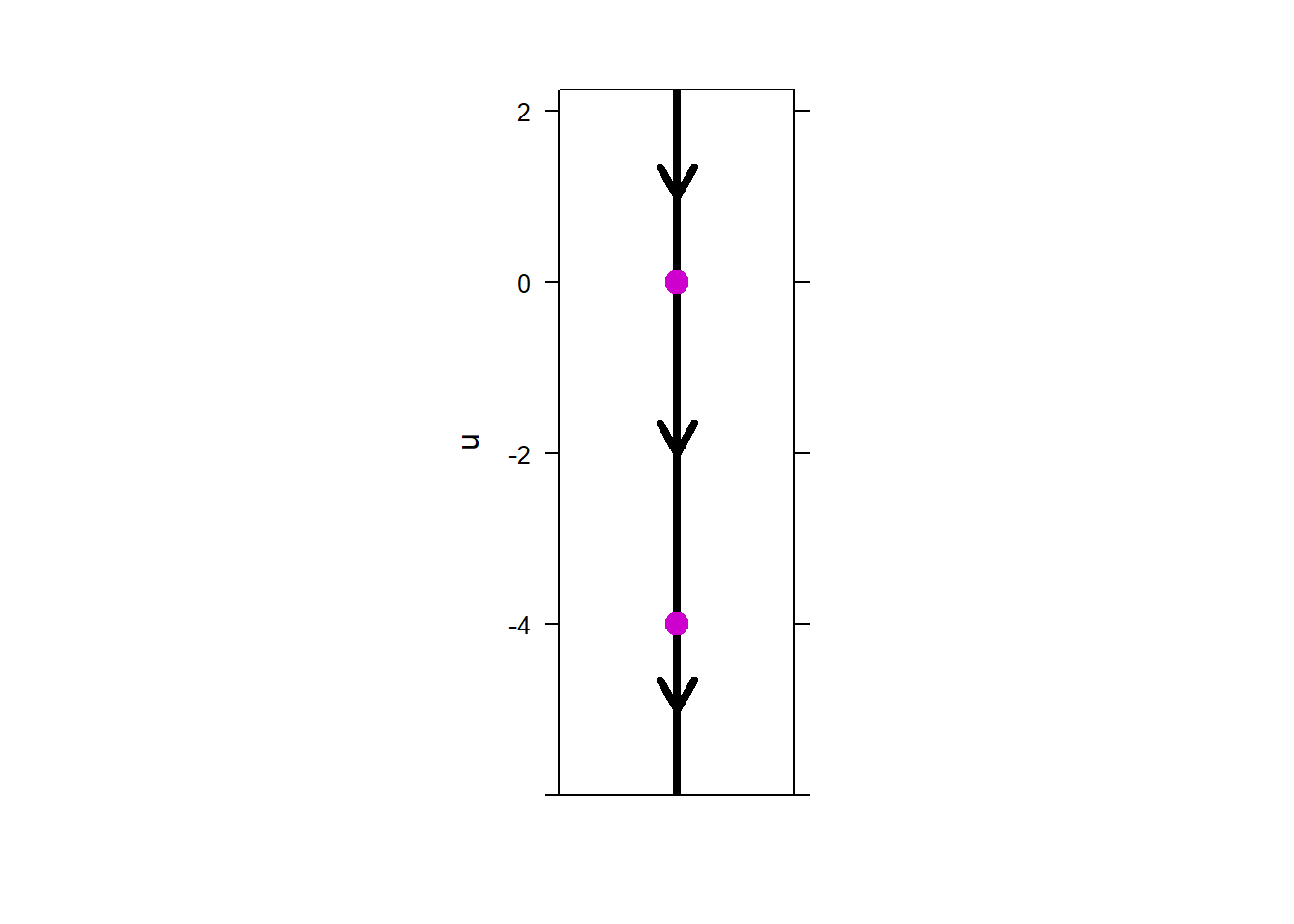
Find the equilibrium solution(s) and plot the phase line for $x' = - 5x^{2} - 20x$.

Start by solving $x' = 0.$

$$\begin{aligned} &- 5x^{2} - 20x = 0\\ &- 5x(x + 4) = 0\end{aligned}$$ The equilibrium solutions are $$x = 0\ \ \text{and}\ \ \ x = - 4.$$ We could also solve this using the quadratic equation or using findZeros.

findZeros(-5*x^2-20*x~x)

##    x
## 1 -4
## 2  0

The equilibrium solutions are $x = - 4$ and $x = 0$. To classify the stability of these solutions, we check the rates of change above and below their values.

$x$	$x'$	Interpretation
$- 5$	$- 5( - 5)^{2} - 20( - 5) = - 25$	Solutions less than -4 are decreasing
$- 2$	$- 5( - 2)^{2} - 20( - 2) = 20$	Solutions between -4 and 0 are increasing
$1$	$- 5(1)^{2} - 20(1) = - 25$	Solutions larger than 0 are decreasing

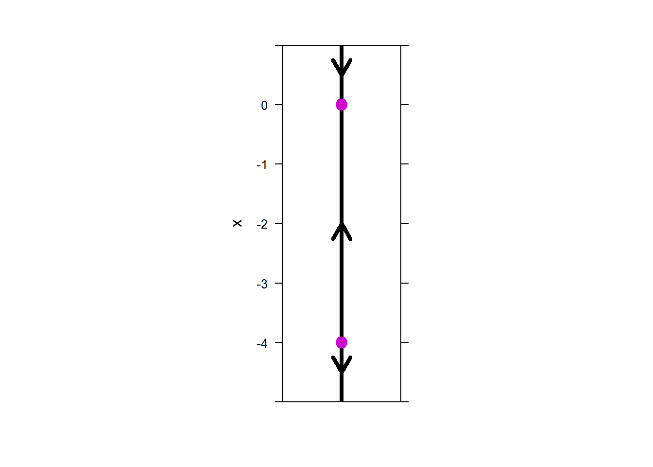
The phase line plot is provided. The phase line shows us that the equilibrium solutions have the following stability:

• $x = - 4$ is unstable

• $x = 0$ is stable

9.2.3 Example 3

Find the equilibrium solution(s) and plot the phase line for $w' = w^2 - 2w + 1$$.

Start by solving $w' = 0.$

$$\begin{aligned} &w^2 - 2w + 1 = 0\\ &(w - 1)^2 = 0. \end{aligned}$$

So, $w=1$ is the only equilibrium solution.

We could also solve this using findZeros.

findZeros(w^2-2*w+1~w)

##   w
## 1 1

To classify the stability of the equilibrium solution, $w = 1$, we check the rates of change above and below the equilibrium value.

$w$	$w'$	Interpretation
$0$	$0^{2} - 2*0 + 1 = 1$	Solutions below 0 are increasing
$2$	$2^{2} - 2*2 + 1 = 1$	Solutions above 0 are increasing

The phase line plot is provided. 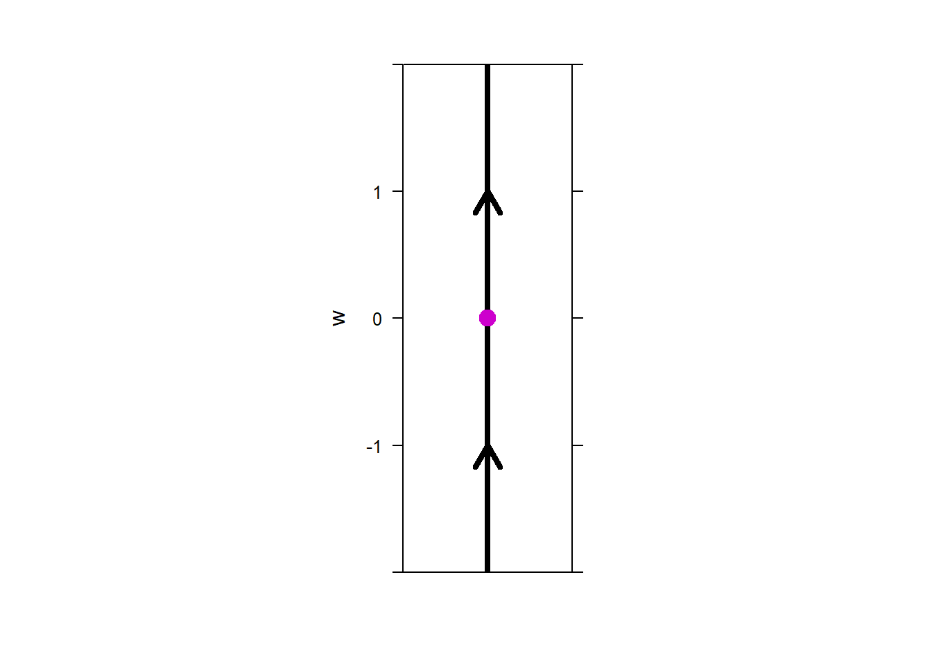The equilibrium solution, $w = 1$, is unstable because some of the solutions near it move away as $t$ increases.

Note: in some textbooks this type of equilibrium solution is called semi-stable.

9.3 Exercises

Problems 1) – 8). For each differential equation: a) find the equilibrium solutions, b) draw the associated phase line, and c) classify the stability of each equilibrium solution.

1)	ODE:	$y^{'} = (y - 4)(y + 1)$
2)	ODE:	$u^{'} = (u + 3)(u - 1)(u - 2)$
3)	ODE:	$w^{'} = w^{2}(1 - w)$
4)	ODE:	$z^{'} = e^{- z}$
5)	ODE:	$y^{'} = - y^{2} + y + 6$
6)	ODE:	$u^{'} = \left( u^{2} + 4u + 4 \right)(1 - u)$
7)	ODE:	$w^{'} = w^{3} - 3w^{2} + 2w$
8)	ODE:	$z^{'} = \sin(z)$

Problems 9) – 12). For each phase line and initial condition: a) identify the equilibrium solutions, b) classify the stability of each equilibrium solution, c) discuss the behavior of the solution corresponding to the given IC, that is, what is the value of the solution that starts at the given initial condtion after a long time?.

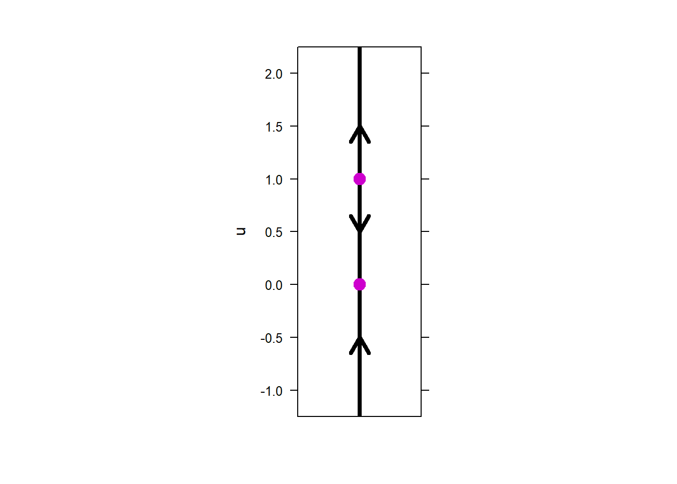
9) Consider the initial conditions $u(0) = 2$, $u(0)=1$, and $u(0)=0.5$.

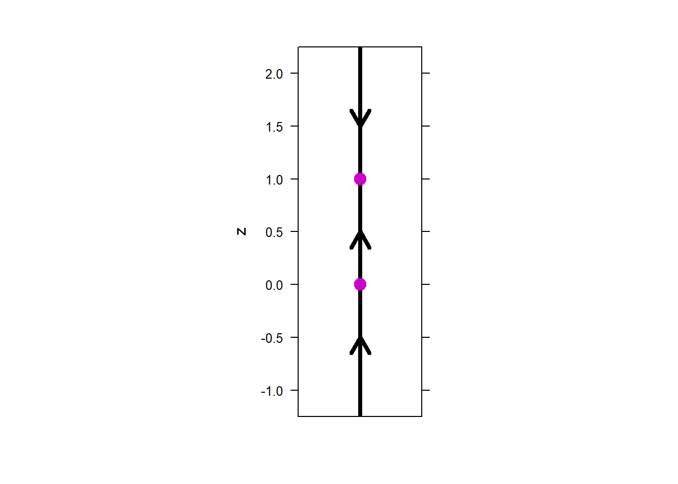
10) Consider the initial condition $z(0) = 1$, $z(0)=0$, and $z(0)=-0.5$.

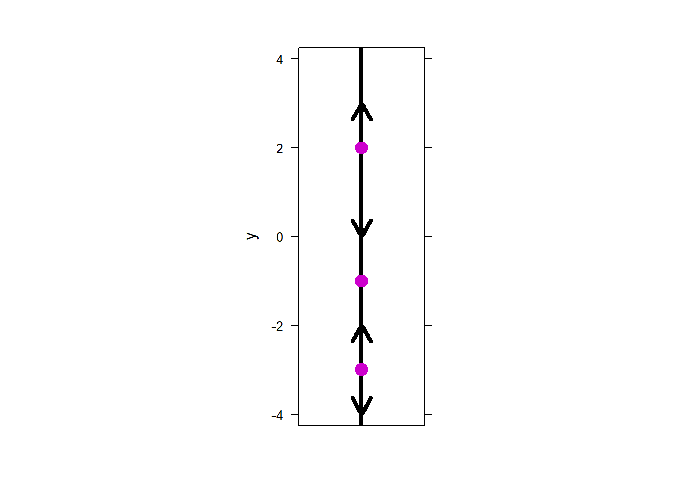
11) Consider the initial condition $y(0) = - 2$, $y(0)=0$, $y(0)=2$, and $y(0)=3$.

12) Consider the initial condition $w(0) = - 5$, $w(0)=-2$, and $w(0)=1$.