Chapter 10 Lesson 35: Modeling with ODEs II

10.1 Note

Today is labeled as a modeling day, but in reality it is about equilibrium solutions, phase lines, and stability. That’s just how things shook out.

10.2 Objectives

Understand the definition of an equilibrium solution and its stability (stable or unstable).
Given a direction field for an ODE, visually estimate the equilibrium solutions of the ODE and determine the stability of each equilibrium.
Given an autonomous first‐order ODE, algebraically solve for the equilibrium solutions of the ODE by hand.
Given an autonomous first‐order ODE, create a phase line and use it to determine the stability of each equilibrium solution.
Given an IVP, describe the long‐term behavior of the solution (as time goes to infinity).

10.3 Reading

Chapter 9 of the Supplemental Reading

10.4 In class

Autonomous ODEs. Start with a reminder that we have been focusing on ODEs of the form $y' = f(y)$ . These are known as autonomous ODEs. In order to find the value of $y'$ , you only need to know the current value of $y$ , not what time it currently is.
Equilibrium Solutions. Define an equilibrium solution as functions that a) solve the ODE, and b) are constant. In order to find equilibrium solutions, we need to solve $0=y'=f(y)$ for $y$ . Since we are looking for constant solutions, these should turn out as constant numbers.
Direction Fields and Phase Lines. Remind them that we can visualize these ODEs using plotODEDirectionField. Recall that autonomous ODE have direction fields that do not change along the $t$ axis, so we can compress all of the information in the direction field into a phase line.
Once we have phase lines, define an equilibrium solution as stable (note, not asymptotically stable) if initial conditions near the equilibrium solution correspond to solutions that stay near the equilibrium solution (don’t tend toward another equilibrium solution, nor $\pm \infty$ ). In the scalar case, that will mean that the solution starting near the equilibrium solution will tend toward the equilibrium solution. Otherwise, the equilibrium solution is unstable.

10.5 R Commands

plotODEDirectionField, findZeros

10.6 Problems & Activities

Start with a fairly simple autonomous ODE, such as $y^{'} = y^{2} - 1$ . Using plotODEDirectionField, note that the behavior of this ODE does not vary based on $t$ . Using $N=21$ as an option puts arrows right on the equilibrium solution. It will look ok if you omit that option.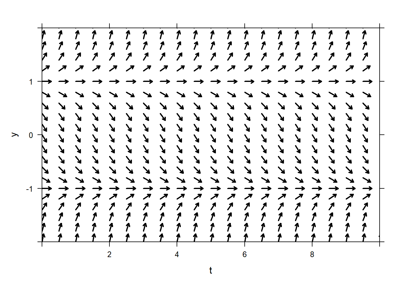
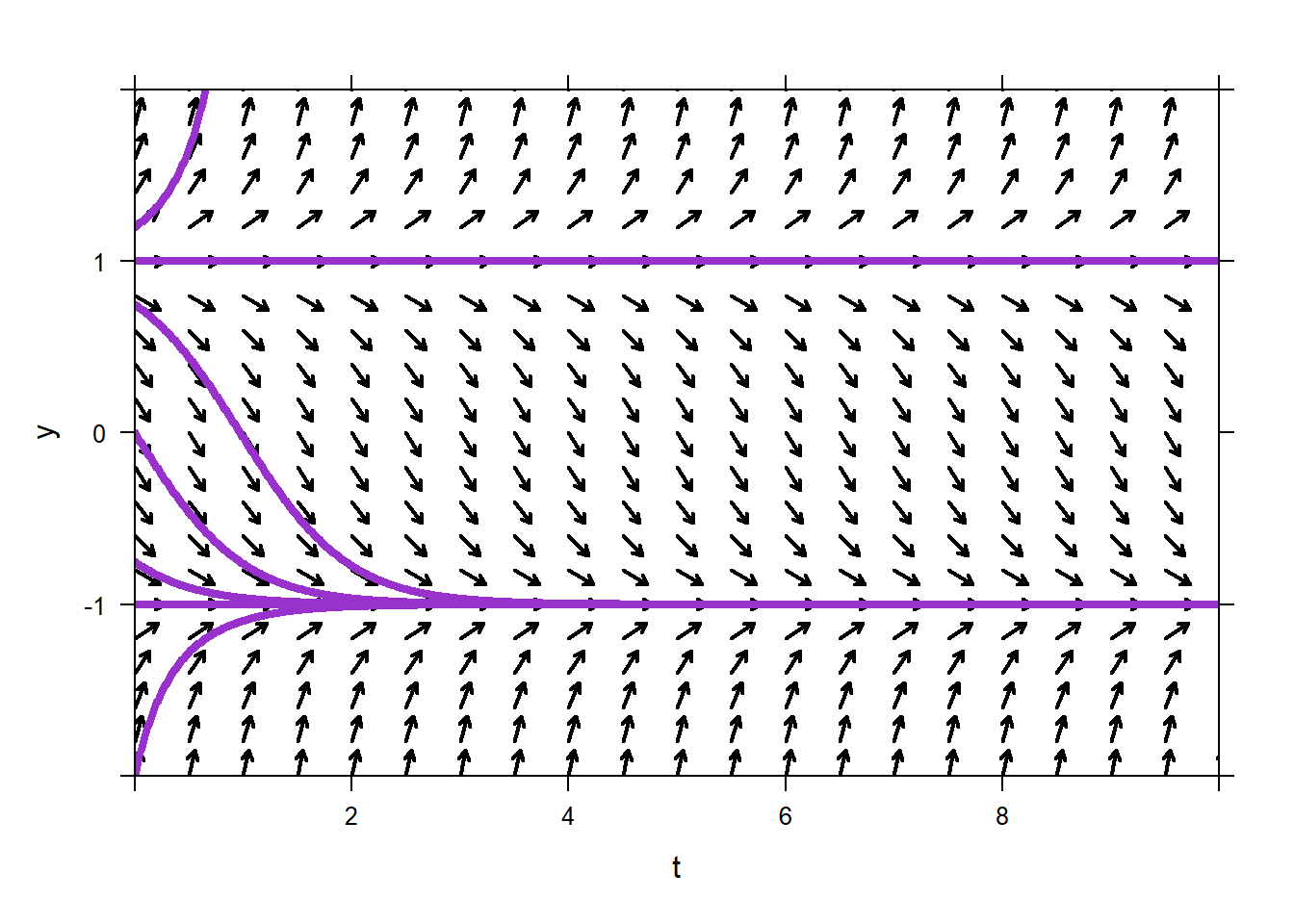
```
plotODEDirectionField(y^2-1~y,ylim=c(-2,2),N=21)
```
Add a few initial conditions to the direction field. Note that they all have one of a few basic behaviors: converge to -1, go to $\infty$ , go to $-\infty$ , and the very special one that stays +1.
```
plotODEDirectionField(y^2-1~y,ylim=c(-2,2),N=21,ics=c(-2,0,-0.75,0.75,1.2,-1,1))
```
Since the behavior of the solutions to autonomous ODEs is so simple, we summarize the information in the direction field with a phase line. Draw a phase line for this ODE.
Note that the initial conditions +1 and -1 were very special and lead to constant solutions. Constant solutions have zero derivative. Constant solutions to the ODE are called equilibrium solutions. To find the equilibrium solutions we could
1. Guess, based off the phase line. Using basic algebra or viewing the direction field or phase line, have the cadets tell you what the equilibrium solutions are for this ODE. In this case, the equilibrium solutions are $y = - 1$ and $y = 1$ .
2. Use algebra. We would need to solve $0=y'=y^2-1$ for $y$ . That would give us $y^2=1$ so $y=\pm 1.$
3. Use findZeros. While this is a little disappointing, it is fine.
```
findZeros(y^2-1~y)
```
```
##    y
## 1 -1
## 2  1
```
There are two types of equilibrium solutions we’ll discuss for autonomous ODEs: stable and unstable. An equilibrium solution is stable if solutions starting nearby stay nearby (doesn’t go to another equilibrium solution, nor $\pm \infty$ . Similarly, an equilibrium solution is unstable if nearby solutions veer away from that equilibrium. Using our example, have the cadets classify $y = - 1$ and $y = 1$ .
If time permits, talk about stability in the context of modeling, say for population models. You could certainly return to the logistic equation example, Example 8.2.0.1 and draw the phase line for that model. Talk about the difference between the stable equilibrium solution at $P=225$ and the unstable one at $P=0$ . Students love considering zombies, so don’t shy away from considering $P<0$ .
The rest of the class should be dedicated to board/group work. There are plenty of exercises in the book.