Chapter 2 Block 2: Optimization

`USAFACalc` for Block 5

There are a lot USAFACalc features that update mosaicCalc functionality that should improve Block 5. Again, everything should be transparent to the student.

2.0.1 `findZeros`

findZeros gets used a lot in this block for finding critical numbers and solving Lagrange multiplier problems.

2.0.1.1 Scalar equations

findZeros is now pretty capable, especially for a single equation. Unlike previous versions, findZeros should now work perfectly when solving any polynomial equation, repeated roots or not. By default it only returns real roots, you can ask for complex by using the option complex=TRUE. That option shouldn’t be needed, but it is there.

findZeros tries to find zeros of an expression. If we want to solve an equation like \[x^7-7x^6+18x^5-30x^4=-35x^3-43x^2+150x-90\] we need to rewrite as \[x^7-7x^6+18x^5-30x^4+35x^3+43x^2-150x+90=0\] and then find the roots of \[x^7-7x^6+18x^5-30x^4+35x^3+43x^2-150x+90.\]

findZeros(x^7-7*x^6+18*x^5-30*x^4+35*x^3+43*x^2-150*x+90~x)

##           x
## 1  1.000000
## 2  3.000000
## 3 -1.414214
## 4  1.414214

The polynomial above factors to $(x-3)^2(x-1)(x^2-2)(x^2+5)$, you can see that findZeros is returning all the roots, including multiplicity, except for the two complex roots $\pm \sqrt{5}i$. If you want those, include complex=TRUE.

findZeros(x^7-7*x^6+18*x^5-30*x^4+35*x^3+43*x^2-150*x+90~x,complex = TRUE)

##                     x
## 1  1.000000+0.000000i
## 2  3.000000+0.000000i
## 3 -1.414214+0.000000i
## 4  1.414214+0.000000i
## 5  0.000000-2.236068i
## 6  0.000000+2.236068i

If the equation is not polynomial, then findZeros will attempt to use Newton’s method with many starting points to find solutions. If there are infinitely many solutions, findZeros will probably find a lot of them, but obviously not all of them. Like any numerical method, findZeros in numerical mode might miss solutions. I’ll detail how to deal with that in these notes. However, we should avoid examples where we need to fiddle with findZeros unless we have a good reason to do so. If the example is really cool in some way, then yes, cajole findZeros to do what you want. If the example is just the first one you thought of, then think of another example.

2.0.1.2 Options to help `findZeros`: `near` and `within`

Solving \[\sin(x)=0\] is done in numerical mode.

solns=findZeros(sin(x)~x)
nrow(solns)

## [1] 821

head(solns)

##            x
## 1 -2125036.1
## 2 -1211033.7
## 3  -980792.7
## 4  -643300.8
## 5  -520992.3
## 6  -452675.2

Here findZeros found 821 solutions, and the ones you probably wanted aren’t near the top.

You can prune down results, and give findZeros a better idea of where to concentrate its effort, by using the options near and within.

findZeros(sin(x)~x,near=0,within = 10)

##        x
## 1 -9.425
## 2 -6.283
## 3 -3.142
## 4  0.000
## 5  3.142
## 6  6.283
## 7  9.425

This gives you the correct results in the interval $(0-10,0+10)$ up to rounding error. By default, numerical mode will round all results to 3 digits, though that can be set with roundDigits option. See ?findZeros.

The default value of within is 100.

It is surprisingly hard to come up with examples where findZeros misses solutions that are in the range $(-100,100)$. We are using a lot of initial starting points. If you happen to find such a case, and you really want to use the example anyway, then using near should get findZeros to find your solution.

findZeros might get fooled into finding solutions that aren’t really there. For instance, consider trying to find critical points of $f(x)=e^{-x^2}$. The only critical point is at $x=0$. However, the derivative gets exceedingly small as $x\to \infty$. If we don’t tell findZeros where to look, it finds 29967 “solutions”, all but one of them spurious. Any numerical solver will get fooled by this. To give a hint, we could use near and within, or just give a range where we are looking with xlim.

f=makeFun(exp(-x^2)~x)
df=D(f(x)~x)

nohint=findZeros(df(x)~x)
nrow(nohint)

## [1] 29967

withhint=findZeros(df(x)~x,xlim=c(-2,2))
withhint

##   x
## 1 0

findZeros is not limited to solving equations with simple expressions. Suppose we want to find a value of $x$ such that \[\text{pnorm}(x)=0.7.\]
No problem, rewrite as \[\text{porm}(x)-0.7=0\] and then invoke findZeros.

findZeros(pnorm(x)-0.7~x)

##       x
## 1 0.524

2.0.2 Solving Systems of Equations with `findZeros`

We can solve systems of equations using findZeros. That will help us a lot with solving constrained optimization problems; we don’t have to stick to super easy problems any more.

Warning: findZeros is literally using Newton’s method with a large number of starting points. By default, it will look for solutions where all components of the solution are within $\pm 100$. It might miss solutions. In my testing, for examples that we are going to use in this class, it seems to work. Just be sure to test it before you do an example in class or assign homework. You can adjust where it looks for solutions using near and within, but only do so if you have a good reason.

Systems of equations are defined using c. Suppose we want to solve \[x^2+y^2=1\] \[\frac 13 x^2+y^2=1.\] First, put the problem in a form similar to the single-variable case: all zeros on the right hand side. \[x^2+y^2-1=0\] \[\frac 13 x^2+y^2-1=0.\] Now we’ll ask R to solve the system of equations, we’ll combine the two expressions using c.

f=makeFun(c(x^2+y^2-1, 1/3*x^2+y^2-1) ~ x&y)
findZeros(f(x,y)~x&y)

##   x  y
## 1 0 -1
## 2 0  1

Suppose we want to solve \[x^2+y^2=1\] \[y=\sin(x).\]

findZeros(c(x^2+y^2-1,
            y-sin(x))~x&y)

##        x      y
## 1 -0.739 -0.674
## 2  0.739  0.674

2.0.3 Plotting functions of two variables, adding constraints

plotFun has been improved to have better resolution, and to allow us to set line width options to make much better figures. I suggest not filling your contour plots unless you have reason to do so, it generally looks bad. Add grid.on if it is useful.

f=makeFun(x^3-8*x+2*y^2~ x & y)
plotFun(f(x,y)~x&y,filled=FALSE,lwd=2,xlim=c(-4,4),ylim=c(-4,4))
grid.on()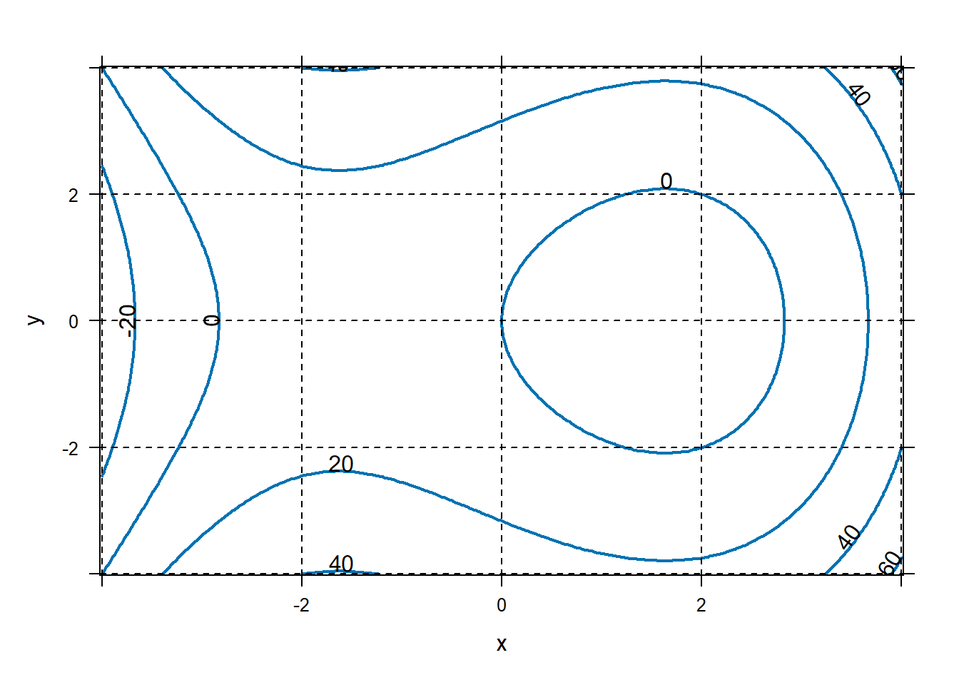

If we are doing constrained optimization, you might want to draw a contour plot of the objective function along with a visualization of the constraint. For example, suppose we want to minimize the objective \[f(x,y)=x^3-8x+2y^2\] subject to the constraint \[\frac 13 (x-2)^2=-(y-2)^2+1.\] To plot the constraint, think of it as the 0-level of the function $g(x,y)=\frac 1 3(x-2)^2 + (y-2)^2-1$, and then plot using the levels option to plotFun. I like to turn off the label on the level curve representing the constraint and add text if helpful.

f=makeFun(x^3-8*x+2*y^2~x&y)
g=makeFun(1/3*(x-2)^2+(y-2)^2-1~x&y)
#Plot a contour plot of f
plotFun(f(x,y)~x&y,xlim=c(-2,5),ylim=c(-2,5),filled=FALSE,col="black",lwd=2)
#add on the constraint, g(x,y)=0
plotFun(g(x,y)~x&y,filled=FALSE,col="firebrick",lwd=3,levels=c(0),labels=FALSE,add=TRUE)
#label the constraint
place.text("constraint",3,0.9,zoom=1.4,col="firebrick")
mathaxis.on()
grid.on()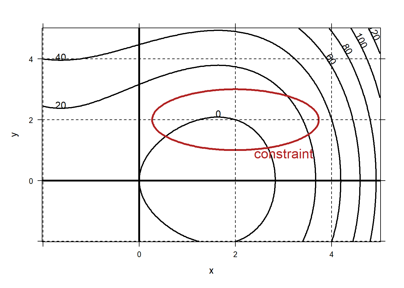

2.0.4 Plotting Vectors and Vector Fields

The function place.vector will add a single vector to your figure. plotVectorField will plot an entire vector field, with vectors scaled to fit on the figure. In this block these functions are good for visualizing gradient vectors.

Vector-valued functions are defined using c. For example, to define the vector-valued function \[F(x,y)=(-y,x)\] use

F=makeFun(c(-y,x)~x&y)
F(2,3)

## [1] -3  2

We can define gradient vectors as follows:

f=makeFun(sin(x*y)~x&y)
fx=D(f(x,y)~x)
fy=D(f(x,y)~y)
Gf=makeFun(c(fx(x,y),fy(x,y))~x&y)
Gf(0,pi)

## [1] 3.141593 0.000000

Consider our function \[f(x,y)=1/10(x^3-8x+2y^2).\] We can create a contour plot of $f$ and visualize its gradient vector at the point (2,2) as below. We can add as many gradient vectors as we like.

Warning Vectors will not look perpendicular to level curves if the aspect ratio of your plot is not 1-1. That doesn’t happen by default. This is, in my opinion, a sneaky thing and it will drive you absolutely crazy until you figure out the problem. You can use asp=1 to force it to happen.

f=makeFun(1/10*(x^3-8*x+2*y^2)~x&y)
plotFun(f(x,y)~x&y,filled=FALSE,col="black",lwd=2,xlim=c(-2,5),ylim=c(-2,5),asp=1)
grid.on()

fx=D(f(x,y)~x)
fy=D(f(x,y)~y)
Gf=makeFun(c(fx(x,y),fy(x,y))~x&y)

place.vector(Gf(2,2),base=c(2,2),col="cadetblue",lwd=2)
place.vector(Gf(4,2),base=c(4,2),col="blueviolet",lwd=2)
place.vector(Gf(0.1,0.63),base=c(0.1,0.63),col="aquamarine4",lwd=2)
place.vector(Gf(2.8,0.47),base=c(2.8,0.47),col="brown4",lwd=2)
place.vector(Gf(1,3.67),base=c(1,3.67),col="darkolivegreen",lwd=2)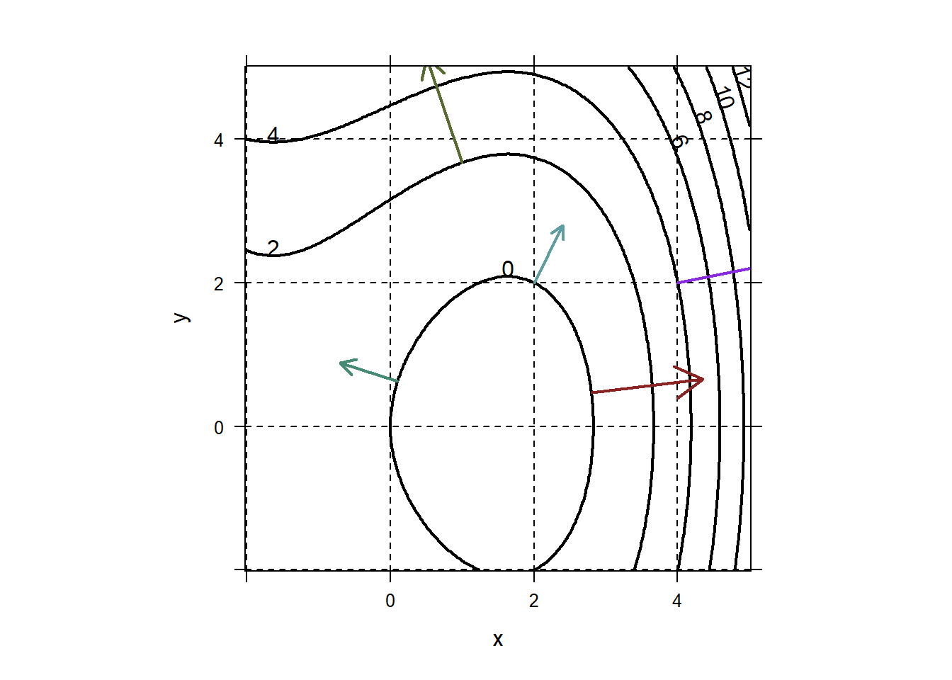

Of course, you might want to plot a whole gradient vector field. You can do that using plotVectorField. plotVectorField scales vectors to fit on the figure reasonably. See the documentation, ?plotVectorField for options.

f=makeFun(1/10*(x^3-8*x+2*y^2)~x&y)
plotFun(f(x,y)~x&y,filled=FALSE,col="black",lwd=2,xlim=c(-2,5),ylim=c(-2,5),asp=1)

fx=D(f(x,y)~x)
fy=D(f(x,y)~y)
Gf=makeFun(c(fx(x,y),fy(x,y))~x&y)

plotVectorField(Gf(x,y)~x&y,add=TRUE,col="darkgoldenrod")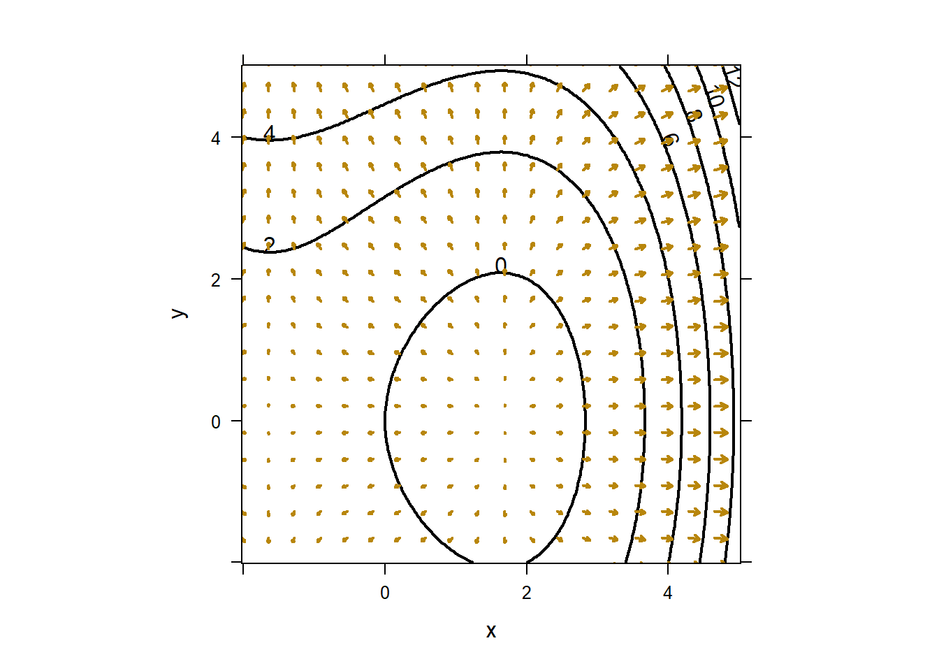

2.0.5 `plotFun` with `surface` option

The plotFun function does a much better job with surfaces than the images in the book. Review plotting surfaces for a refresher.

f=makeFun(3*(1-x)^2*exp(-(x^2)-(y+1)^2)- 10*(x/5 - x^3 - y^5)*exp(-x^2-y^2)
          - 1/3*exp(-(x+1)^2 - y^2)~x&y)
plotFun(f(x,y)~x&y,xlim=c(-3,3), ylim=c(-3,3),surface=TRUE)

2.1 Lesson 18: Extreme Values & Critical Numbers I

2.1.1 Objectives

Understand the definitions of critical number and global extrema (global max/min).
Given the plot of a function on a specified interval, identify any critical numbers and global extrema, including value and location, or state why they do not exist.
Given a function, use the derivative of the function to find all critical numbers of the function, by hand and using R.
Describe the Extreme Value Theorem and under what conditions it applies.
Given a function on a closed interval, find the global extrema, including value and location, by hand and using R.

2.1.2 Reading

Section 5.1.

2.1.3 In Class

Global Extreme Values. This entire block is about optimization, which is identifying where a function has extreme values (minimum or maximum). Note that there is a difference between global and local extreme values. We will cover local extreme values next lesson, but there’s no need to shy away from the definition of local extreme values in today’s lesson.
Extreme Value Theorem. What the cadets need to understand is that if a function is continuous over a domain, it has a global minimum and global maximum. Just like with the integration, I have no idea why the book wants to keep saying smooth.
Critical Numbers. The Extreme Value Theorem doesn’t tell us how to find global extrema. Critical numbers will help us identify those values. Let’s all get on the same page here with our terminology. I use the term critical number to refer to the input value(s) where the derivative is zero or undefined. I use critical point to refer to the full coordinates (input and output value). Cadets should have the opportunity to look at a few plots of functions to visually identify these critical points. Note that for some non-smooth functions, we can still identify global extreme values (like $f\left( x \right) = \left| x \right|$).
Using the Derivative to Find Critical Numbers. It’s not always feasible, necessary or efficient to plot a function to search for critical numbers. We can simply find the derivative of a function and find where that function is equal to zero (or undefined). Cadets should have the opportunity to take a function, find its derivative, set equal to zero, and solve for critical numbers. They should also be able to identify whether each critical number is a minimum or a maximum.

2.1.4 R Commands

makeFun, plotFun, D, findZeros

2.1.5 Problems & Activities

Start with an example using a polynomial function. Consider the function $f\left( x \right) = 6x^{4} - 8x^{3} - 24x^{2}$.
1. Define the function in R and plot it on the domain $\lbrack - 2,\ 3\rbrack$.
```
f = makeFun(6*x^4-8*x^3-24*x^2~x)
plotFun(f(x)~x,xlim=range(-2,3),lwd=2)
mathaxis.on()
grid.on()
```
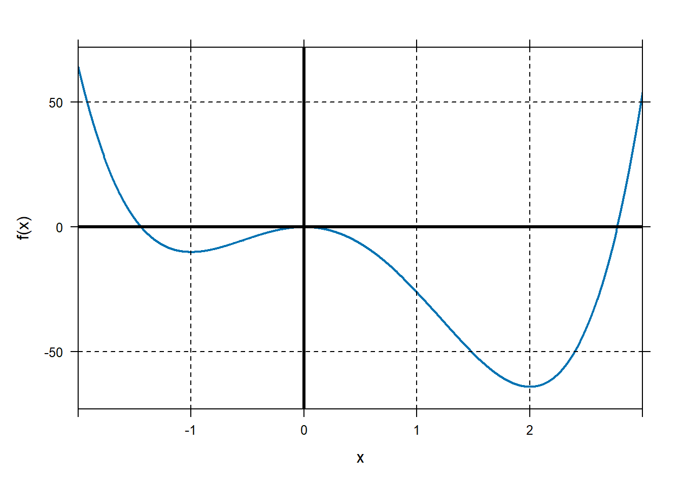
2. Note that because this is a polynomial function, it is differentiable across all values of $x$. Thus, by the extreme value theorem, it has a global minimum and global maximum in the domain $\lbrack - 2,\ 3\rbrack$. Graphically, we can approximate these values. We can also identify the critical numbers.
3. Let’s find the critical numbers of $f(x)$ on our domain. Recall from the reading that critical numbers are values of $x$ where the derivative is equal to zero or does not exist. Again, since this is a polynomial, the derivative exists at all values of $x$, so we need to find where the derivative is equal to 0. We can do this by hand. \[f^{'}\left( x \right) = 24x^{3} - 24x^{2} - 48x = 0\] Factoring: \[24x\left( x^{2} - x - 2 \right) = 24x\left( x - 2 \right)\left( x + 1 \right) = 0\] So, the critical numbers are $x = - 1,\ \ x = 0$, and $x = 2$. We could also use findZeros in R:
```
Df=D(f(x)~x)
findZeros(Df(x)~x)
```
```
##    x
## 1 -1
## 2  0
## 3  2
```
4. Use the critical numbers to determine the global maximum and minimum of $f(x)$ on the domain $\lbrack - 2,\ 3\rbrack$. This involves evaluating the function at the critical numbers and the endpoints of the interval. We can do this by hand or using R.
```
c(f(-1), f(0), f(2), f(-2), f(3))
```
```
## [1] -10   0 -64  64  54
```
  The global maximum occurs at $x = - 2$ and $f\left( - 2 \right) = 64$. The global minimum occurs when $x = 2$ and $f\left( 2 \right) = - 64$.
5. You should also point out the values $x = - 1$ and $x = 0$ represent local extreme values. We’ll explore this next time, but cadets are likely to ask why these values aren’t global extreme values.
Exercises 51-78. They should visualize each function and ID extreme values.

2.2 Lesson 19: Extreme Values and Critical Numbers II

2.2.1 Objectives

Understand the definition of local extrema (local max/min).
Given the plot of a function, identify all local extrema, including value and location.
Given a function, use the first derivative test to determine whether each critical number is the location of a local maximum, local minimum, or neither, by hand and using R.
Given the plot of a function’s derivative, identify any critical numbers and the locations of any local extrema for the original function.

2.2.2 Reading

Section 5.2.

2.2.3 In Class

Local Extreme Values. Some of this should be review from last time. Distinguish between global and local extreme values using a function as an example. Speculate as to how we could tell (in the absence of a plot) whether a critical number is a local minimum or local maximum.
First Derivative Test. Cadets should recognize that at a local extreme value, the derivative changes sign from positive to negative (for a maximum) or from negative to positive (for a minimum). Demonstrate this with our example, using “by-hand” methods and using R.

2.2.4 R Commands

makeFun, plotFun, D, findZeros

2.2.5 Problems & Activities

Start with our example from last time. (The function $f\left( x \right) = 6x^{4} - 8x^{3} - 24x^{2}$ on the domain $\lbrack - 2,\ 3\rbrack$).
1. Define and plot this function in R. Remind them where the global extreme values are located.
```
f = makeFun(6*x^4-8*x^3-24*x^2~x)
plotFun(f(x)~x,xlim=range(-2,3),lwd=2); grid.on(); mathaxis.on()
```
```
Df=D(f(x)~x)
findZeros(Df(x)~x)
```
```
##    x
## 1 -1
## 2  0
## 3  2
```
```
c(f(-2),f(-1),f(0),f(2),f(3))
```
```
## [1]  64 -10   0 -64  54
```
  We found the global maximum at the left endpoint, $x = - 2$ and $f\left( - 2 \right) = 64$. We found the global minimum at $x = 2$ and $f\left( 2 \right) = - 64$.
2. Now let’s distinguish between global and local extreme values. Graphically, we can see that in addition to the value $x = 2$, there are two other critical numbers ($x = - 1$, $x = 0$) that represent local extreme values. While we can see that the value $x = - 1$ is at a local minimum and the value $x = 0$ is at a local maximum, we can also tell by inspecting the derivative, which represents rate of change. Just to the left of $x = - 1$, the function is decreasing (negative derivative). The function flattens out at $x = - 1$ then begins to increase. Similar behavior is seen at $x = 0$ and $x = 2$.
  
  Plot the derivative of $f(x)$ to demonstrate this.
```
f = makeFun(6*x^4-8*x^3-24*x^2~x)
Df=D(f(x)~x)
plotFun(f(x)~x,xlim=range(-2,3),lwd=2,col="blue"); grid.on(); mathaxis.on()
plotFun(Df(x)~x,add=TRUE,col="red",lwd=2)
place.text("f(x)",1.2,-23,zoom=1.4,col="blue")
place.text("f'(x)",2,-23,zoom=1.4,col="red")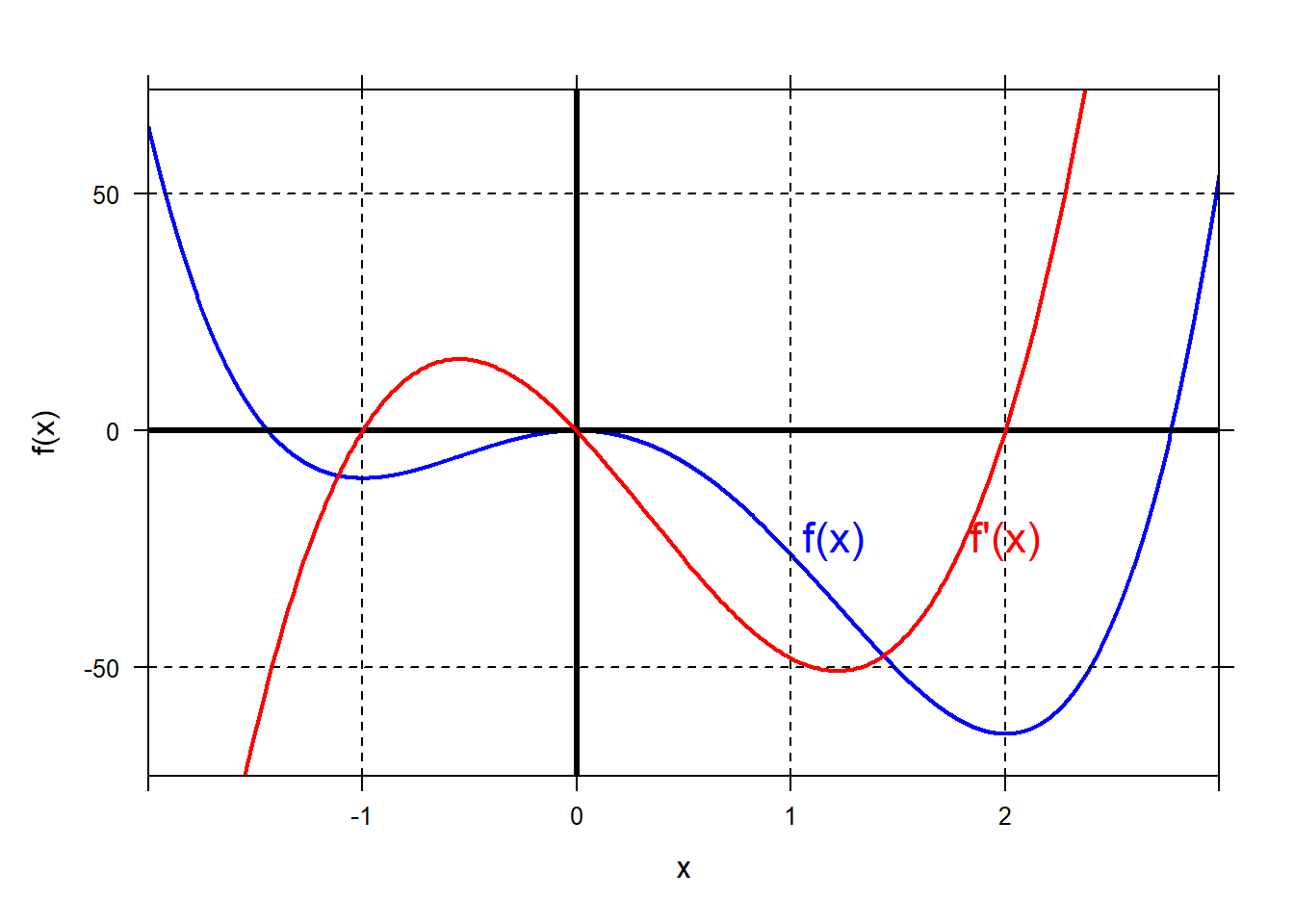
```
  We can see that at local extreme values, $f^{'}\left( x \right) = 0$. We can also use $f'(x)$ to determine whether the local extreme value is a minimum or maximum by looking at values of $f'$ near the critical number.
```
c(Df(-1.1),Df(-0.1),Df(1.9),Df(-0.9),Df(0.1),Df(2.1))
```
```
## [1]  -8.184   4.536 -13.224   6.264  -5.016  15.624
```
  As an example, for the critical number $x = - 1$, we see that just to the left of that value, $f^{'}\left( - 1.1 \right) < 0$, and just to the right of that value, $f^{'}\left( - 0.9 \right) > 0$. Because the rate of change went from negative to positive, we know that a local minimum exists at $x = - 1$.
  
  Speculative question: What if we have a critical number, and the sign of the derivative is the same on either side? We’ll explore this next time.
Take a look at Exercise 5 in Section 5.2. This is an example of a non-smooth function that has local extreme values at critical numbers where the derivative does not exist. We don’t spend a lot of time on these types of functions, but it’s important to identify extreme values even in non-smooth functions.
Exercises 41-54, Section 5.2.

2.3 Lesson 20: Concavity and Extreme Values

2.3.1 Objectives

Understand the definitions of concavity (concave up/down) and inflection points.
Given the plot of a function’s first derivative, identify where the original function is concave up, concave down, and the locations of any inflection points.
Given a function, use its second derivative to determine concavity and to identify any points of inflection.
Given a function, use the second derivative test to determine whether each critical number is the location of a local maximum, local minimum, or if the test is inconclusive.

2.3.2 Reading

Section 5.3.

2.3.3 In Class

Review. We have introduced the concept of concavity in prior lessons both this semester and last semester. The point of this lesson is to emphasize the role of concavity in determining type of extreme value.
Concavity and First Derivative. When determining whether a critical number is at a maximum or minimum, it is helpful to know whether the function is concave up or down. We can determine concavity by exploring the first derivative. When a function’s first derivative is increasing, it is concave up. When a function’s first derivative is decreasing, it is concave down. Demonstrate with an example.
Concavity and Second Derivative. Since the second derivative describes how the first derivative changes, we can use that to determine concavity. When the first derivative is increasing, the second derivative is positive, and the function is concave up. And vice-versa.
Points of Inflection. An inflection point occurs when the function switches from concave up to concave down or vice-versa. Remember that at an inflection point, the second derivative must equal zero. However, the second derivative equaling zero does not necessarily imply an inflection point (e.g. $f(x)=x^4$ has no inflection point at $x=0$).
Putting it Together. The rest of the time should be dedicated to practice. Given a function, use the concavity of the function to determine whether a critical number is a local minimum, a local maximum, or an inflection point.

2.3.4 R Commands

makeFun, plotFun

2.3.5 Problems & Activities

Start with the function $f\left( x \right) = x^{3} - 5x$ and plot on the domain $\lbrack - 3,\ 3\rbrack$.
```
f=makeFun(x^3-5*x~x)
plotFun(f(x)~x,xlim=range(-3,3),lwd=2)
mathaxis.on()
grid.on()
```
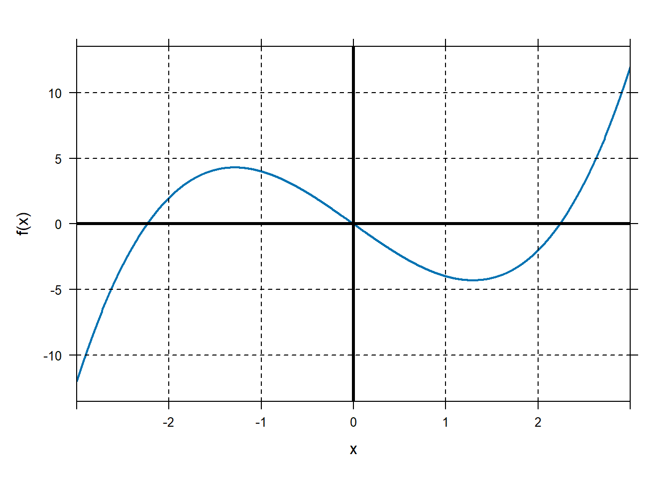Find the critical numbers of this function.

Critical numbers occur when $f'\left( x \right)$ is equal to 0 or undefined.

\[f'\left( x \right) = 3x^{2} - 5 = 0\]

Thus, critical numbers are $x = \pm \sqrt{\frac{5}{3}} \approx \pm 1.291$.

We could also use R:
```
Df=D(f(x)~x)
zeros = findZeros(Df(x)~x)
zeros
```
```
##           x
## 1 -1.290994
## 2  1.290994
```
What kind of local extreme values are these critical numbers? To find out, let’s figure out the concavity at each critical number. We can do this in two ways: with the first derivative and with the second derivative.

First derivative: Looking at $f'(x)$ near our critical numbers:
```
c(Df(-1.291-0.1), Df(-1.291+0.1), Df(1.291-0.1), Df(-1.291+0.1))
```
```
## [1]  0.804643 -0.744557 -0.744557 -0.744557
```
For $x = - 1.291$, the first derivative is decreasing. Thus it is concave down at this point.

For $x = 1.291$, the first derivative is increasing and the function is therefore concave up.

Second derivative: We can also determine whether $f''(x)$ is positive or negative at our critical numbers:
```
DDf=D(Df(x)~x)
c(DDf(-1.291), DDf(1.291))
```
```
## [1] -7.746  7.746
```
For $x = - 1.291$, the second derivative is negative. Thus the function is concave down at this point.

For $x = 1.291$, the second derivative is positive and the function is therefore concave up.

Based on the concavity at our critical numbers, we conclude that $x = - 1.291$ is at a local maximum and $x = 1.291$ is at a local minimum.
For the same function, identify any points of inflection.

We can do that by finding where $f^{''}\left( x \right) = 0$.
```
findZeros(DDf(x)~x)
```
```
##   x
## 1 0
```
$f''(0)=0$, so $x = 0$ is a potential inflection point. You can check by seeing if $f''(x)$ switches sign near 0.
```
c(DDf(0-0.1),DDf(0+0.1))
```
```
## [1] -0.6  0.6
```
$f''(x)$ does switch signs at $x=0$, so we have an inflection point.
Section 5.3, Exercises 27-66.

2.4 Lesson 21: Newton’s Method I

2.4.1 Objectives

Understand and write the formula for Newton’s Method for a given function, in recursive notation and in function notation.
Given a function, use Newton’s Method to approximate a zero of the function near a specified input.
Given a function, use Newton’s Method to approximate a critical number of the function near a specified input.

2.4.2 Reading

Section 5.4.

2.4.3 In Class

Review of Critical Numbers and Function Behavior. Start with an example where they have to find local extreme values and inflection points using derivatives. Emphasize that the key to finding critical numbers is finding where the derivative of the function is equal to 0.
Newton’s Method. Introduce a function for which zeros are hard to find algebraically. We could use findZeros, but how does that function find solutions? The answer is (similar to) Newton’s Method, an iterative technique for solving an equation. Introduce the algorithm and explain it intuitively. Next, demonstrate (by hand) its use on our function.
Newton’s Method for Optimization. Now introduce a function for which critical numbers are hard to obtain algebraically. Find the zeros of the derivative using Newton’s Method. Emphasize that we are finding the zeros of the derivative, so we’ll need to find the derivative of the derivative.

2.4.4 R Commands

makeFun, plotFun, D

2.4.5 Problems & Activities

Let $f\left( x \right) = x^{3} - 6x^{2} + 9x + 2$. Find any local extreme values and inflection points. \[f^{'}\left( x \right) = 3x^{2} - 12x + 9\] Setting this equal to zero, we can find the critical numbers: \[3x^{2} - 12x + 9 = \left( 3x - 3 \right)\left( x - 3 \right) = 0.\] So, our critical numbers are $x = 1$ and $x = 3$. Alternatively, we could have done this in R.
```
f=makeFun(x^3-6*x^2+9*x+2~x)
Df=D(f(x)~x)
findZeros(Df(x)~x)
```
```
##   x
## 1 1
## 2 3
```
We can use the second derivative test to try to determine the type of critical points we have. \[f^{''}\left( x \right) = 6x - 12\] $f^{''}\left( 1 \right) = - 6 < 0$, implying that $x = 1$ is at a local maximum. $f^{''}\left( 3 \right) = 6 > 0$ so $x = 3$ is at a local minimum. Also, note that $f^{''}\left( 2 \right) = 0$, $f''(2-0.1)=-0.6$, $f''(2+0.1)=0.6$, so $f$ has an inflection point at $x=2$.
Above, we were able to factor to find the zeros of our derivative. What if our function is not as easy to solve algebraically. For example, find the zeros of the function $g\left( x \right) = x^{2} + \sin\left( x \right)$. I don’t know how to do this algebraically. Instead, we’ll use Newton’s Method. We’ll start with an initial guess at the root, $x_0$. From $x_0$, we’ll improve our guess, and call the next guess $x_1$. From $x_1$ we’ll compute another guess, $x_2$, and so on.

Take a look at our example:
```
g=makeFun(x^2+sin(x)~x)
plotFun(g(x)~x,xlim=range(-3,3),lwd=2)
grid.on()
mathaxis.on()
```
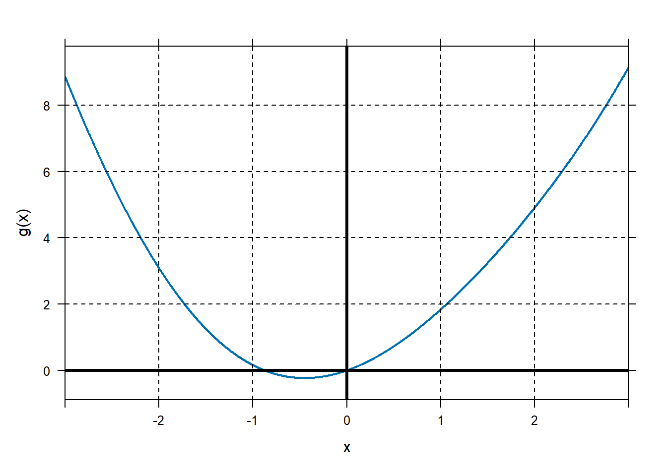It looks like this function has a zero near $x = - 1$. For demonstration, let our initial guess be $x_{0} = - 2$. Let’s construct the tangent line to the graph of $g$ at $x_0=2$. A point on that line is

\[(x_0,g(x_0))=(-2,g(-2))=(-2,3.09).\] The derivative of $g$ is \[g'(x)=2x+\cos(x)\] and so the slope of our tangent line is \[g'(-2)=-4.42.\] Using point-slope form, we find that the equation of the tangent line is \[y-3.09 = -4.42(x-(-2))\] or equivalently \[y = -4.42(x-(-2))+3.09.\] We can calculate these things and plot the resulting tangent line in R. in R:
```
g=makeFun(x^2+sin(x)~x)
y0=g(-2)
Dg=D(g(x)~x)
slope=Dg(-2)
tanline=makeFun(slope*(x-(-2))+y0~x)
plotFun(tanline(x)~x,add=T,col="red",lwd=2,lty="dashed")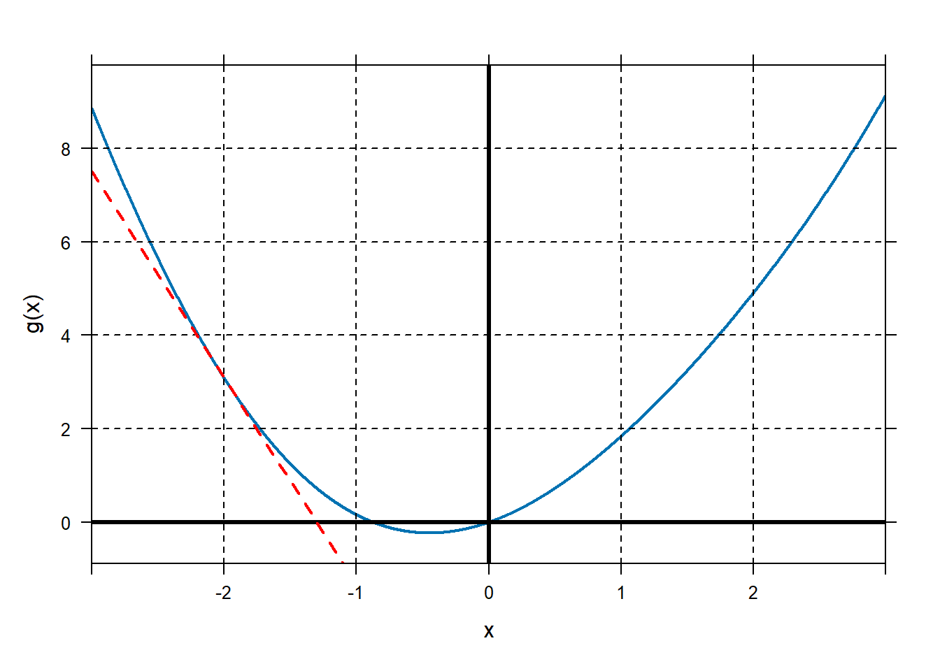
```
One of the big ideas of calculus is that the graph of the tangent line to $g$ will stay pretty close to the graph of $g$ for a little bit near the point of tangency. We are looking for where the graph of $g$ crosses the $x$-axis, instead, we’ll figure out where the graph of the tangent line crosses the $x$-axis. The tangent line is useful because a) it stays close to the graph of $g$ for a little bit, and b) linear functions are easy to work with.

We’ll figure out where the graph of the tangent line crosses the $x$-axis, and then we’ll use that as our improved estimate of the root of $g$.

The equation of our tangent line is \[y = -4.42(x-(-2))+3.09.\] At the point where the tangent line crosses the $x$-axis, \[0 = -4.42(x-(-2))+3.09.\] We can solve for the $x$ coordinate. \[x=\frac{-3.09}{ -4.42}+(-2) = -1.3.\]

Great, our new guess at the root is $x_1 = -1.3$. There is nothing stopping us from repeating this process. \[g(x_1)=g(-1.3)=0.73\] \[g'(x_1)=g'(-1.3)=-2.33\] So the equation of this tangent line is \[y-0.73=-2.33(x-(-1.3)).\] This tangent line crosses the $x$-axis at \[x_2=-1.3 - \frac{0.73}{-2.33}=-0.99.\] The pattern emerging is that our $k^{th}$ estimate of the root of $g$ is calculated as \[x_{k}=x_{k-1}-\frac{g(x_{k-1})}{g'(x_{k-1})}.\] Repeat a few times, following the general workflow below. Either build the figure as you go, or just show the completed figure at the end. Notice that, in this case, we do indeed keep getting closer and closer to our desired root of $g$.
```
g=makeFun(x^2+sin(x)~x)
plotFun(g(x)~x,xlim=c(-3,3),lwd=2)
grid.on()
mathaxis.on()


Dg=D(g(x)~x)
x0=-2;
place.text("x0",x0,-0.5,col='magenta')

tanlinex0=makeFun(g(x0)+Dg(x0)*(x-x0)~x)
plotFun(tanlinex0(x)~x,add=T,col="red",lwd=2,lty="dashed")

x1=x0-g(x0)/Dg(x0)
x1
```
```
## [1] -1.300136
```
```
place.text("x1",x1,-0.5,col="magenta")
tanlinex1=makeFun(g(x1)+Dg(x1)*(x-x1)~x)
plotFun(tanlinex1(x)~x,add=T,col="red",lwd=2,lty="dashed")

x2=x1-g(x1)/Dg(x1)
x2
```
```
## [1] -0.9886105
```
```
place.text("x2",x2,-0.5,col="magenta")
tanlinex2=makeFun(g(x2)+Dg(x2)*(x-x2)~x)
plotFun(tanlinex2(x)~x,add=T,col="red",lwd=2,lty="dashed")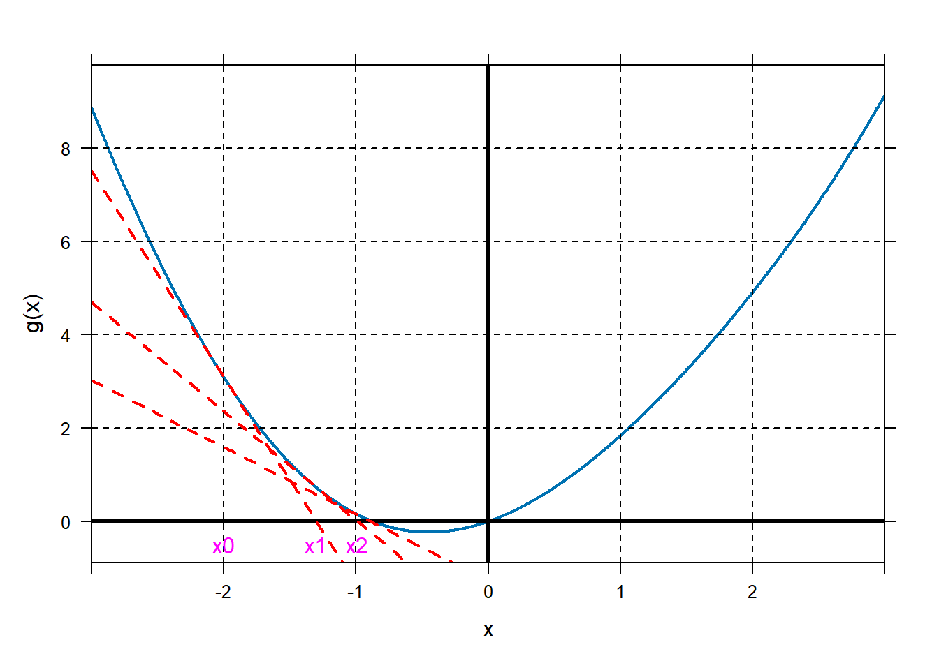
```
```
x3=x2-g(x2)/Dg(x2)
x3
```
```
## [1] -0.8890652
```
```
x4=x3-g(x3)/Dg(x3)

x4
```
```
## [1] -0.8769102
```
It looks like our estimates of the root are settling down to a consistent answer, about $-0.88$. If we check, $g(x_4)=2.0491711\times 10^{-4}$, pretty close to being 0!
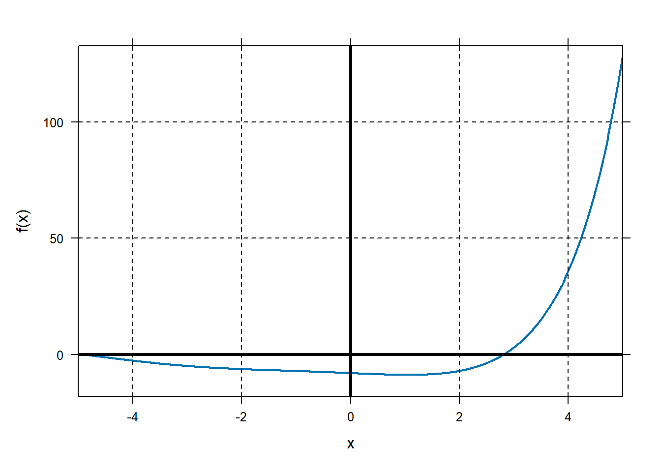
Application to optimization. Let $f\left( x \right) = e^{x} + \cos\left( x \right) - 2x-10$. Use five iterations of Newton’s method to find any critical numbers of this function.

Note that critical numbers occur when $f^{'}\left( x \right) = 0$ or is undefined. So we need to apply Newton’s Method to $f'(x)$. Start with $x_{0} = 2$.

\[x_{n + 1} = x_{n} - \frac{f^{'}\left( x_{n} \right)}{f''(x_{n})}\]

Note, it is also totally fine to just define $g(x)=f'(x)$ and then do Newton’s method from above.
```
f=makeFun(exp(x)+cos(x)-2*x-10~x)
plotFun(f(x)~x,xlim=range(-5,5),lwd=2); mathaxis.on(); grid.on();
```
```
x0=2

Df=D(f(x)~x)
D2f=D(Df(x)~x)

x1=x0-Df(x0)/D2f(x0)
x2=x1-Df(x1)/D2f(x1)
x3=x2-Df(x2)/D2f(x2)
x4=x3-Df(x3)/D2f(x3)
x5=x4-Df(x4)/D2f(x4)
c(x1,x2,x3,x4,x5)
```
```
## [1] 1.426055 1.134193 1.058807 1.054144 1.054127
```
A good estimate of that critical point is near $x_5 = 1.05$.
If there’s still time, have them practice with Exercises 25-38 from section 5.4.

2.5 Lesson 22: Newton’s Method II

2.5.1 Objectives

Use the Iterate command in R to implement Newton’s Method.
Given two functions, use Newton’s Method to approximate where the graphs of the functions intersect.
Given an equation, use Newton’s Method to approximate a solution of the equation.
Given a function or equation, use a plot to determine an appropriate initial value to implement Newton’s Method for the desired zero, critical number, intersection, or solution.

2.5.2 Reading

Section 5.4.

2.5.3 In Class

Review of Newton’s Method for Optimization. Start with an example and have them use Newton’s Method to find critical numbers of a function. When going through this example, note that we can build another function in R to make our lives a little easier.
Using Iterate. Return to that example and demonstrate how to use the Iterate function to automate this process. Note that this function does not appear in the text.
Examples. Give the rest of the class to practice. Cadets should know how to implement Newton’s Method in R and should be able to describe/implement a step of Newton’s Method by hand.

2.5.4 R Commands

makeFun, plotFun, D, Iterate

2.5.5 Problems & Activities

Let $f\left( x \right) = x^{3}\ln\left( x \right) - x^{2}$. Use five iterations of Newton’s Method to find a critical number of this function near $x = 2$.

f=makeFun(x^3*log(x)-x^2~x)

plotFun(f(x)~x,xlim=range(0,3),lwd=2,col="darkseagreen4"); grid.on(); mathaxis.on()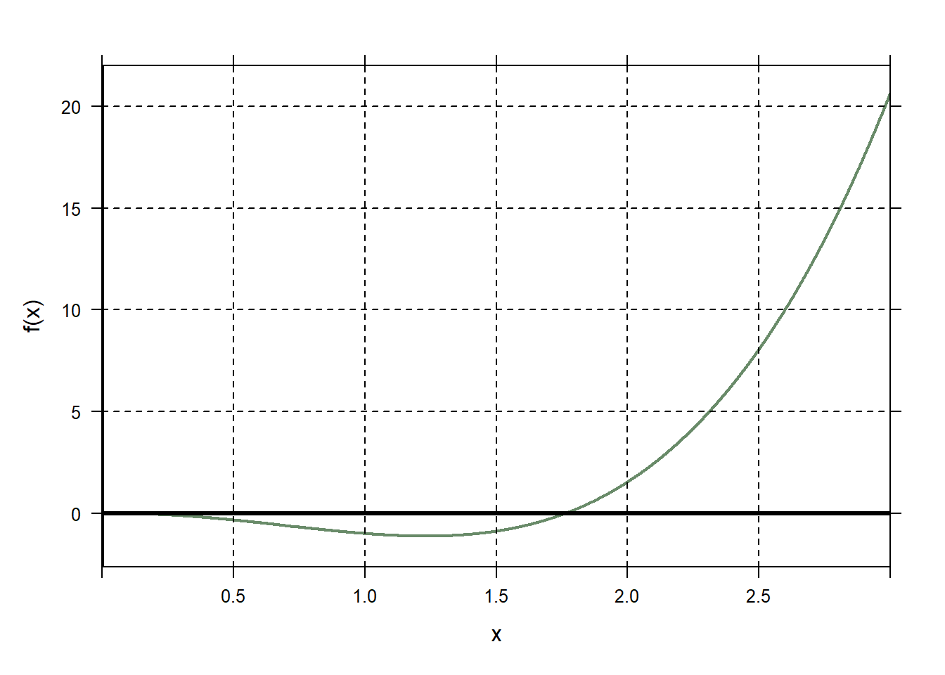

Df=D(f(x)~x)
D2f=D(Df(x)~x)

x0=2
x1=x0-Df(x0)/D2f(x0)
x2=x1-Df(x1)/D2f(x1)
x3=x2-Df(x2)/D2f(x2)
c(x0,x1,x2,x3)

## [1] 2.000000 1.490263 1.279760 1.233636

We can automate the repetitive typing above. Instead of repeating this over and over while incrementing the label of$x$, let’s define a function NM:

NM=makeFun(x-Df(x)/D2f(x)~x)
x0=2
x1=NM(x0)
x2=NM(x1)
x3=NM(x2)
x4=NM(x3)
x5=NM(x4)

c(x0,x1,x2,x3,x4,x5)

## [1] 2.000000 1.490263 1.279760 1.233636 1.231329 1.231323

Besides saving some work, defining a function NM allows us to use another tool specifically for repeatedly evaluating a function on the last output. We can use the Iterate function to apply a function over and over again:
```
Iterate(NM(x)~x, x0 = 2, n = 5)
```
```
##   n        x
## 1 0 2.000000
## 2 1 1.490263
## 3 2 1.279760
## 4 3 1.233636
## 5 4 1.231329
## 6 5 1.231323
```
Note the syntax for this function: first is the tilde expression for the function. We also need to specify the starting value, x0=2, and the number of iterations n=5. Note that in our case, we reached a consistent value within 5 iterations.
The rest of the class should be dedicated to practice: Exercises 55-64, 75-86, Section 5.4. Note that some problems ask the student to find zeros of a function while others ask for local extreme values.

2.6 Lesson 23: Multivariable Optimization

2.6.1 Objectives

Given the contour plot of a function with two inputs, estimate the locations and values of any local extrema.
Use partial derivatives to find the critical points of a function with two inputs, by hand or using R.
Given a function with two inputs, use the multivariable second derivative test to determine whether each critical point is the location of a local maximum, local minimum, saddle point, or if the test is inconclusive.

2.6.2 Reading

Section 5.5.

2.6.3 Special Notes

DFMS (Dr. Stanhope) has 3-D printed surfaces that are very helpful (and fun) for this lesson and the next one.

We don’t have to stick to super-simple systems of equations – findZeros is pretty useful here. Note that this is not done in the book.

2.6.4 In Class

Multivariable Functions. Start with a reminder of multivariable functions. We last discussed these when covering partial derivatives at the end of the last semester. Emphasize that just like functions with one input, we can use differentiation to locate local extreme values of functions with two inputs. This simply involves taking the partial derivative of the function with respect to each input individually and finding the values of the input for which BOTH derivatives are equal to zero. These values constitute “critical points” which are the multivariable analog to “critical numbers.”
Second Derivative Test. Just like with functions with one input, we can use the second derivative to determine the type of critical point (minimum, maximum, saddle point).
Global Extreme Values. The text extensively goes through how to find global extreme values in specified regions. Cadets should understand that in order to find global extreme values, we would need to find the critical points and check the boundary of the region, but specific application of this topic will wait until Math 243.
The intention is for students to use findZeros to find critical points, rather than solving systems of equations.

2.6.5 R Commands

makeFun, plotFun, D, findZeros

2.6.6 Problems & Activities

Start with Question 1 on Page 555 in the text. Take a moment to remind how to read a contour plot. This function has a local maximum of about 7 at about $\left( 2,1 \right)$. It has another local maximum of about 3 near the point $( - 0.25,\ 0.25)$. It has a local minimum of about -1 near the point $(1, - 1)$.
We can also plot contour plots with R. Consider the function $f\left( x,y \right) = x^{3} - 8x + {2y}^{2}$. Plot this function on the domain $x = \lbrack - 4,4\rbrack$ and $y = \lbrack - 3,3\rbrack$. Use this plot to approximate the local extreme values.
```
f=makeFun(x^3-8*x+2*y^2~ x & y)
plotFun(f(x,y)~x&y,xlim=range(-4,4),ylim=range(-3,3),
        filled=FALSE,lwd=2,levels=c(-20,-10,-8,-5,0,5,8,10,20));
grid.on()
```
You can plot this function as a surface also.
```
plotFun(f(x,y)~x&y,xlim=range(-4,4),ylim=range(-3,3),surface=TRUE);
```
It looks like this function has a local minimum of about $- 8$ near the point $(1.5,0)$ and a point that is neither a minimum nor a maximum but is otherwise unusual near the point $( - 1.5,0)$. More on this later.
In order to find these values exactly, we can use differentiation to find and classify critical points (in the multivariable case, we refer to critical points rather than critical numbers). For a function with two inputs, a critical point is an input where both first derivatives are equal to 0. So for our example, we want $x$ and $y$ such that \[\frac{\partial}{\partial x}f\left( x,y \right) = 3x^{2} - 8 = 0\] and \[\frac{\partial}{\partial y}f\left( x,y \right) = 4y = 0\]
```
Dfx=D(f(x,y)~x)
Dfy=D(f(x,y)~y)
critpoints=findZeros(c(Dfx(x,y),Dfy(x,y))~x&y)
critpoints
```
```
##        x y
## 1 -1.633 0
## 2  1.633 0
```
```
plotFun(f(x,y)~x&y,xlim=range(-4,4),ylim=range(-3,3),filled=FALSE,lwd=2,
        levels=c(-20,-10,-8,-5,0,5,8,10,20));
#pch is the character for the dots.  You can use 1-25 for different 
#symbols, or put any charcter like "+".  
#
#cex is the character expansion, like zoom. 
plotPoints(y~x,data=critpoints,add=TRUE,pch=19,col="magenta1",cex=1.3)
grid.on()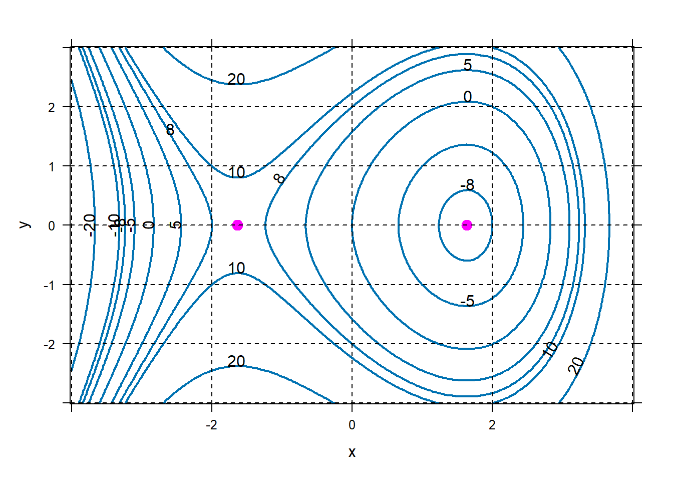
```
We can see that critical points are where $x = \pm \sqrt{\frac{8}{3}} \approx \pm 1.633$ and $y = 0$. This is consistent with what we see on the contour plot.
We have two critical points: $(-1.633,0)$ and $(1.633,0)$. But how do we know if these represent mins, maxs, or something else? In the single variable case, we would use the second derivative. But when dealing with two variables, there are three types of second derivatives: the second derivative with respect to $x$, $f_{xx}$, the second derivative with respect to $y$, $f_{yy}$, and the mixed derivative $f_{xy} = f_{yx}$. The multivariable second derivative test (page 558) helps us classify critical points in functions with two inputs. The requires we find the “discriminant”, $D(a,b)$ of the function.

For our function, we note that $f_{xx}(a,b) = 6a$, $f_{yy}(a,b) = 4$ and $f_{xy}(a,b) = 0$. So \[D\left( a,b \right) = 24a.\]

For our critical point $\left( 1.633,0 \right)$, \[D\left( 1.633,0 \right) = 24\cdot 1.633 = 39.192 > 0.\] Since $f_{xx}\left( 1.633,0 \right) = 6\cdot 1.633 > 0$, this critical point is a local minimum of $f$.

For our critical point $( - 1.633,0)$, \[D\left( - 1.633,0 \right) = 24\cdot(-1.633) < 0.\] Thus, this critical point is a “saddle point” (think Pringles).

Spend some time looking at the surface plot and contour plot above to interpret saddle points.
Find all the critical points of $f(x,y)=x^4+y^4-4xy+1$. Classify the critical points.

First, find the critical points.
```
f=makeFun(x^4+y^4-4*x*y+1~x&y)
fx=D(f(x,y)~x)
fy=D(f(x,y)~y)
findZeros(c(fx(x,y),
            fy(x,y))~x&y)
```
```
##    x  y
## 1 -1 -1
## 2  0  0
## 3  1  1
```
Make a graph of the function, see what the second derivative test should tell you.
```
plotFun(f(x,y)~x&y,xlim=c(-2,2),ylim=c(-2,2),lwd=2,filled=FALSE,
        levels=c(-0.8,-0.5,0,1,2,3,10,20,30));
grid.on()
plotPoints(c(-1,0,1)~c(-1,0,1),add=TRUE,pch=19,cex=1.3,col="maroon")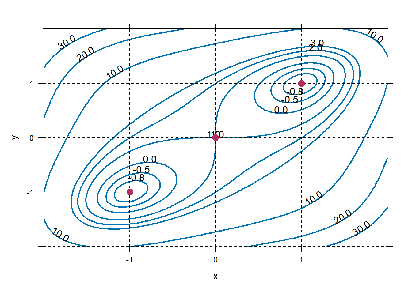
```
Looks like $(1,1)$ and $(-1,-1)$ should be local minima, and $(0,0)$ a saddle point. Compute the second derivative test. Watch out if you name your discriminant D, you will overwrite the differentiate command.
```
fxx=D(f(x,y)~x&x)
fyy=D(f(x,y)~y&y)
fxy=D(f(x,y)~x&y)

Disc=makeFun(fxx(x,y)*fyy(x,y)-fxy(x,y)^2~x&y)
c(Disc(0,0),Disc(-1,-1),Disc(1,1))
```
```
## [1] -16 128 128
```
Second Derivative Test is telling us that $(0,0)$ is a saddle point. It is telling us that $(-1,-1)$ and $(1,1)$ are something. Now we can check.
```
c(fxx(1,1),fxx(-1,-1))
```
```
## [1] 12 12
```
So the second derivative test is telling us that we have local minima, as expected.
Do a couple of exercises 47-58, or make up your own similar ones. Warning: findZeros is likely to not perform well with exponential functions whose derivatives tend toward zero, I’d avoid those.
Focus on 65-68. Emphasize writing down the objective function from a word problem.

2.7 Lesson 24: Constrained Optimization I

2.7.1 Objectives

Given a multivariable function, compute the gradient vector, by hand or using R.
Understand and describe the properties of the gradient vector.
Given a contour plot of a multivariable function, approximate the location and value of a local extreme subject to a given constraint.

2.7.2 Reading

Section 5.6.

2.7.3 In Class

Review & Constrained Optimization. Start this lesson with a review of optimization of multivariable functions. No example problem needed, but remind them that in order to find and classify local extreme values, we need to find where both partial first derivatives are equal to zero AND conduct the multivariable second derivative test. In the next two lessons, we will focus on optimization subject to a constraint. A motivating example could be that a company’s profits are a function of its expenditures on parts and labor. However, according to its budget, it can only spend so much total on parts and labor.
The Gradient Vector. In order to address these problems, we will need to work with gradient vectors and Lagrange multipliers. First, introduce the gradient vector and have them practice obtaining the gradient vector for various multivariable functions.
Lagrange Multiplier. Introduce the Lagrange multiplier as a measure of how much a local extreme value changes when the constraint is adjusted. For example, if the company raises its budget by a certain amount, how much will its maximum profit increase?
Visually Approximating Solutions. Finish up with visually approximating extreme values and the Lagrange multiplier for specific examples. If there’s time, you can introduce analytical solutions, but we will focus on that next class.

2.7.4 R Commands

makeFun, plotFun, D, findZeros

2.7.5 Problems & Activities

Start with a quick reminder from last time that we need to use partial derivatives and the multivariable second derivative test to find and classify local extreme values for multivariable functions (no example required). Today, we will focus on optimization subject to a constraint. As a motivating example, consider a company whose profits are a function of its expenditures on parts and labor. However, it has a budget (a constraint on expenditures).
Before we can address this problem, we need to introduce two new concepts: the gradient vector and the Lagrange multiplier. The gradient vector (denoted by $\nabla f(x,y)$) is simply the vector of partial derivatives. At a particular input point, the gradient vector represents the direction and magnitude of steepest ascent from that point. As an example, consider the function $f\left( x,y \right) = x^{3} - 8x + 2y^{2}$. For this function, \[\nabla f\left( x,y \right) = \begin{pmatrix} 3x^{2} - 8 \\ 4y \\ \end{pmatrix}\]

Note that the gradient of $f(x,y)$ is a vector-valued function. In other words, the gradient of $f$ depends on the value of $\text{x\ }$and$\text{\ y}$. For example, at $x = 2$ and $y = 0$,

\[\nabla f\left( 2, 0 \right) = \begin{pmatrix} 3\cdot 2^{2} - 8 \\ 4\cdot 0 \\ \end{pmatrix} = \begin{pmatrix} 4 \\ 0 \\ \end{pmatrix}\]

This means that at the point $\left( 2,0 \right)$, the direction of steepest ascent is along the vector $\begin{pmatrix} 4 \\ 0 \\ \end{pmatrix}$.

Similarly, \[\nabla f(1,1)=\begin{pmatrix} 3\cdot 1^2 -8 \\ 4\cdot 1\end{pmatrix}=\begin{pmatrix} -5\\4 \end{pmatrix}.\] So, the direction in which $f$ is increasing most rapidly from $(1,1)$ is in the direction of $(-5,4)$.

Let’s examine this visually:
```
f=makeFun(x^3-8*x+2*y^2~ x & y)
plotFun(f(x,y)~x&y,xlim=range(-6,6),ylim=range(-6,6),filled=FALSE,
        asp=1,lwd=2,levels=c(-20,-8,-5,0,10,20,30,50))
grid.on()
place.vector(c(4,0),base=c(2,0),col="deeppink4")
place.vector(c(-5,4),base=c(1,1),col="maroon")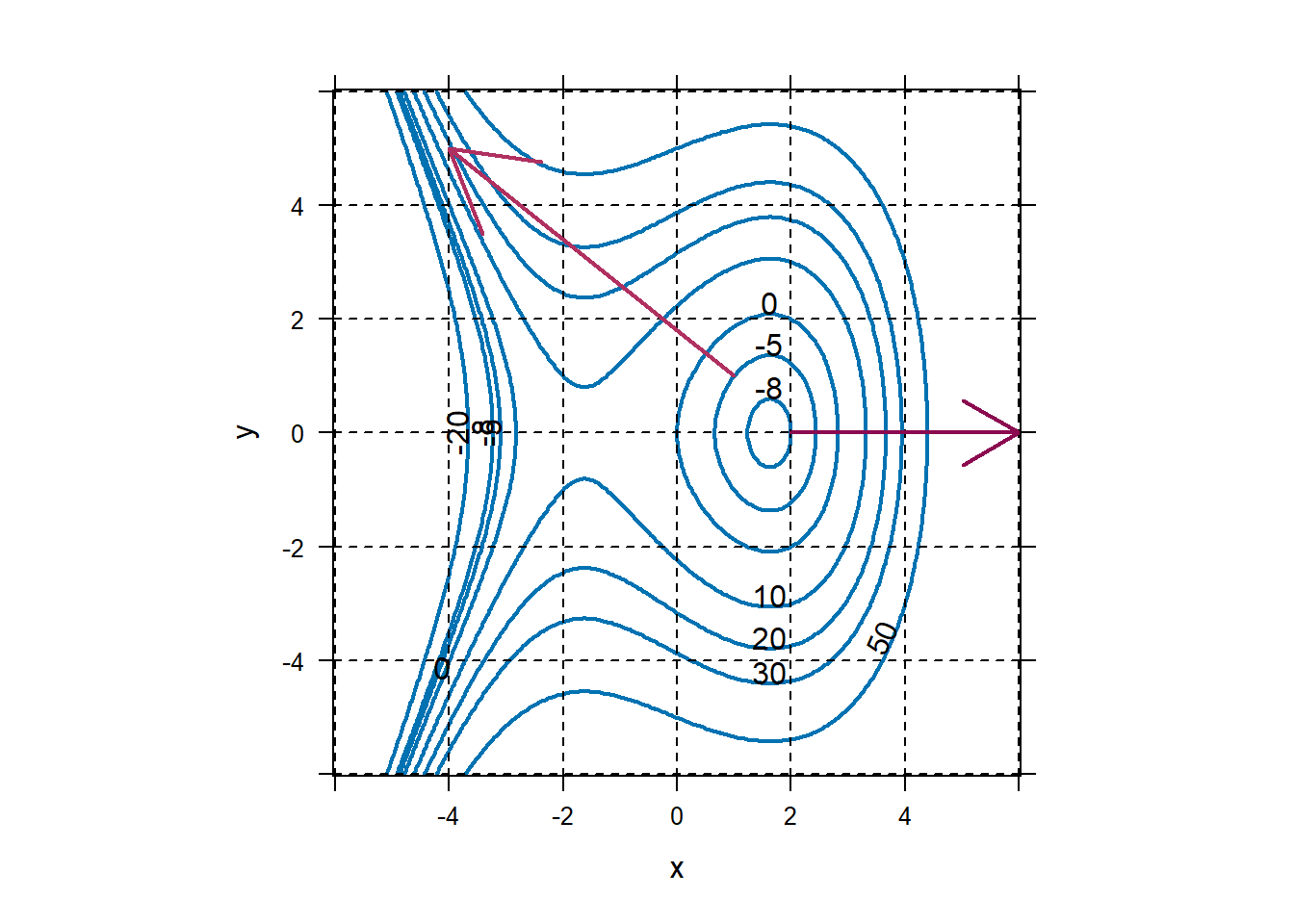
```
Notice that gradient vectors always point to higher-value level curves. Note also that gradient vectors are always perpendicular to the level curve from which they emanate.
Cadets should spend the next few minutes practicing how to obtain a gradient vector and how to interpret it at specific inputs. For exercises 15-18, have them find the gradient vector at the inputs. They don’t need to use R to plot the gradient vector, but they should use it to plot the function.
There is nothing wrong with following the book starting on 575. At this stage, students should just be looking at the pictures. I’m going to take this opportunity to demonstrate creating contour plots and constraints so that we can create our own material for GRs, slides, etc. Consult any standard calculus text for functions with “interesting” shapes. Consider the function \[f(x,y)=10x^2y-5x^2-4y^2-x^4-2y^4,\] whose graph is shown below.
```
f=makeFun(10*x^2*y-5*x^2-4*y^2-x^4-2*y^4~x&y)
plotFun(f(x,y)~x&y,xlim=c(-3,3),ylim=c(-2,3),filled=FALSE,lwd=2,
        levels=c(-0.1,-0.7,-1.5,-3  ,-10,-20,-30,3,7))
grid.on()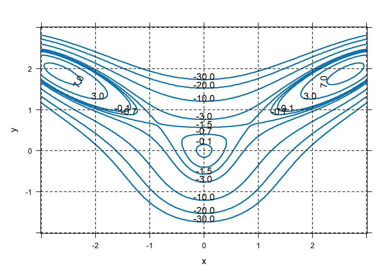
```
1. Approximate any local extreme values. Just by visual inspection, we can see that the function has two local maximums with values a bit over 7 near $(2.5,1.9)$ and $(-2.5,1.9)$. It has a local maximum at $(0,0)$ with a value of a bit over $-0.1$. It also has two saddle points near $(\pm 0.9,0.7)$.
```
dfx=D(f(x,y)~x)
dfy=D(f(x,y)~y)
cps=findZeros(c(dfx(x,y),dfy(x,y))~x&y)
cps
```
```
##        x     y
## 1 -2.644 1.898
## 2 -0.857 0.647
## 3  0.000 0.000
## 4  0.857 0.647
## 5  2.644 1.898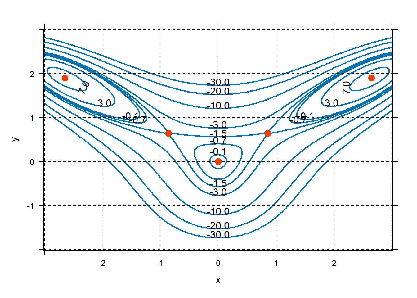
```
```
plotPoints(y~x,data=cps,pch=19,cex=1.3,add=TRUE,col="orangered2")
```
2. Now suppose we are only interested in evaluating $f$ at inputs that also satisfy $x+y=-0.2$. This is called constrained optimization. The function $f$ is called the objective function, and $x+y=-0.2$ is called the constraint. Now what are the local extreme values?
```
f=makeFun(10*x^2*y-5*x^2-4*y^2-x^4-2*y^4~x&y)
g=makeFun(x+y~x&y)
plotFun(f(x,y)~x&y,xlim=c(-3,3),ylim=c(-2,3),filled=FALSE,
  lwd=2,levels=c(-0.1,-0.7,-1.5,-3,-10,-20,-30,3,7))
plotFun(g(x,y)~x&y,filled=FALSE,lwd=2,levels=-0.2,
  add=TRUE,col="deeppink",labels=FALSE)
place.text("x+y=-0.2",x=1.7,y=-1.5,col="deeppink")
grid.on()

#Find constrained extreme values. 
dfx=D(f(x,y)~x); dfy=D(f(x,y)~y);
dgx=D(g(x,y)~x); dgy=D(g(x,y)~x);
cps=findZeros(c(dfx(x,y)-l*dgx(x,y), 
                dfy(x,y)-l*dgy(x,y), 
                g(x,y)+0.2)~x&y&l)
cps
```
```
##        x      y       l
## 1 -1.960  1.760 -19.271
## 2 -0.858  0.658  -0.181
## 3 -0.082 -0.118   1.021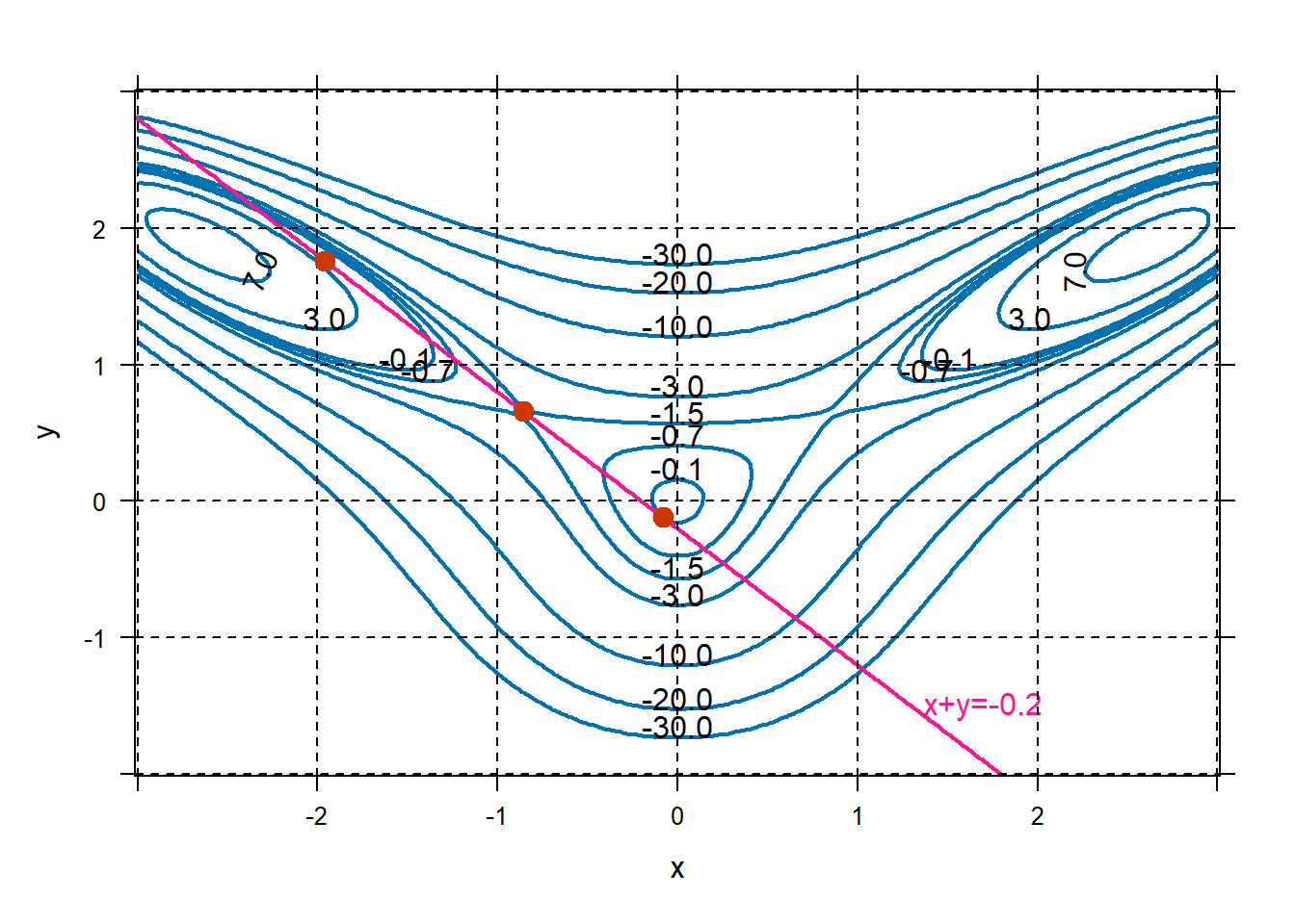
```
```
plotPoints(y~x,data=cps,add=TRUE,pch=19,cex=1.3,
  col="orangered3")
```
  Starting at the top left of the constraint and walking toward the right, we see that the values of $f$ along the constraint start out small, near $-30$, and increase rapidly to nearly $3$ around the point $(-1.9,1.7)$. Value of $f$ then starts decreasing to about $-1.5$ around $(-0.9,0.7)$, and then starts increasing to about $-0.1$ around $(-0.1,-0.1)$. After that, the function $f$ decreases. So we have three local extrema for this constrained problem. \[\text{Point: } (-1.9,1.7) \text{ Value: } 2.9 \text{ Type: Local Max}\] \[\text{Point: } (-0.9,0.7) \text{ Value: } -1.5 \text{ Type: Local Min}\] \[\text{Point: } (-0.1,-0.1)\text{ Value: } -0.1 \text{ Type: Local Max}\]
3. What if the constraint changed? If we change the value of the constraint to -0.5 instead of -0.2. How would each of these local extremes change?
```
cps=findZeros(c(dfx(x,y)-l*dgx(x,y), 
                dfy(x,y)-l*dgy(x,y), 
                g(x,y)+0.5)~x&y&l)
print(cps)
```
```
##        x      y       l
## 1 -2.385  1.885 -11.802
## 2 -0.926  0.426   4.547
## 3 -0.189 -0.311   3.088
```
```
plotFun(g(x,y)~x&y,add=TRUE,col="paleturquoise3",
  filled=FALSE,levels=-0.5,lwd=2)
place.text("x+y=-0.5",0.8,-1.8,col="paleturquoise3")
plotPoints(y~x,data=cps,add=TRUE,pch=19,
  cex=1.3,col="palegreen3")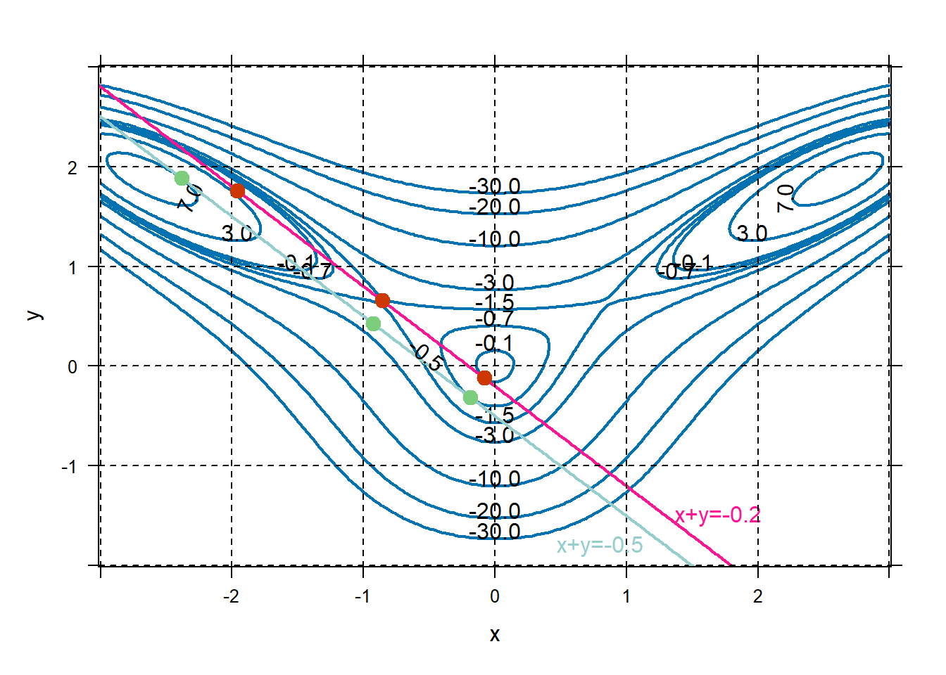
```
  We can see that now we have the following local extrema: \[\text{Point: } (-2.4,1.9)\text{ Value: } 7.0 \text{ Type: Local Max}\] \[\text{Point: } (-0.9,0.4)\text{ Value: } -2.16 \text{ Type: Local Min}\] \[\text{Point: } (-0.2,0.3)\text{ Value: } -0.7 \text{ Type: Local Max}\]
4. The Lagrange multiplier, $\lambda$, measures the rate of change in our local extreme values per unit of change to the constraint. \[\frac{\text{change in extreme value}}{\text{change in constraint value}}\approx \lambda.\]
  Technically, $\lambda$ is the value of this quantity as the change in constraint goes to 0.
  
  Regarding the local max in the top-left, our extreme value changed to $7.0$ from $2.9$, when the constraint changed to $-0.5$ from $-0.2$. Thus an approximation of the Lagrange multiplier associated with the local maximum at $(-2.4,1.9)$ is \[\lambda \approx \frac{7.0-2.9}{-0.5-(-0.2)} = -5.86.\]
  
  Regarding the “middle” local minimum, the extreme value changed to $-2.2$ from $-1.5$ when the constraint changed to $-0.5$ from $-0.2$. So an approximation of the Lagrange multiplier associated with the local maximum at $(-0.9,0.7)$ is \[\lambda \approx \frac{-2.2-(-1.5)}{-0.5-(-0.2)} = 1.\] Regarding the right-most extreme value, the value changed to $-0.7$ from $-0.1$ when the constraint changed to $-0.5$ from $-0.2$. So an approximation to the Lagrange multiplier associated with the local maximum at $(-0.1,-0.1)$ is \[\lambda \approx \frac{-0.7-(-0.1)}{-0.5-(-0.2)} = 0.86.\]
The rest of the time should be dedicated to approximating and interpreting Lagrange multipliers graphically. I recommend Example 4 on page 576, Question 3 on page 577, and exercises 31-38. Next time, we’ll talk about how to use Lagrange multipliers to find exact solutions. If you wish to make your own figures, which will be nicer looking than those of the book, use the Examples on pages 578-581 as source.

2.8 Lesson 25: Constrained Optimization II

2.8.1 Objectives

Given a multivariable function and a constraint, write out the system of equations for the method of Lagrange multipliers.
Given a point and corresponding lambda value, determine if the system of equations is satisfied for the method of Lagrange multipliers.
Use the method of Lagrange multipliers to find the location and/or value of all local extrema subject to a given constraint, by hand or using R.
Interpret the value of the Lagrange multiplier in the context of the problem.

2.8.2 Reading

Section 5.6.

2.8.3 In Class

Review of Constrained Optimization. Start with a reminder that we are considering multivariable optimization under constraints. Go through an example where they visually approximate the local extreme values and the Lagrange multiplier.
Method of Lagrange Multipliers. First, try to get the intuition for the method of Lagrange Multipliers using the linked CalcPlot3d activity. Then, solve several examples.
Students may use findZeros to solve the Lagrange multiplier system of equations. Be careful with your examples, findZeros might miss solutions or get tricked into finding extraneous solutions.

The rest of this lesson should be spent on the method of Lagrange multipliers to find analytical solutions to constrained optimization problems. Emphasize that this requires keeping track of two multivariable functions (the function itself and the constraint function). Also emphasize that this will be a little more involved than what we’re used to so will require a lot more practice.

2.8.4 R Commands

makeFun, plotFun, D, findZeros

Problems & Activities

Start with an example from Exercises 31-38 as a reminder of what is a Lagrange multiplier and how to approximate it graphically.
Build the intuition. Here is a CalcPlot3D visualization of a constrainted optimization problem. A contour plot of $f$ is in red, the constraint is in red.
1. Have them look at the graph and idenfity the extreme values.
2. Use the checkmarks in the toolbar on the left to highlight the critical points that they found.
3. Use the slider at the bottom of the screen to move the highlighted point around the constraint. From the highlighted point, the gradient of $f$ is shown in red, the gradient of $g$ is shown in blue.
4. Note that at the critical points, the gradient of $f$ and the gradient of $g$ are parallel. Therefore, at critical points, $\nabla f = \lambda \nabla g$, for some value of $\lambda$. It turns out that yes, the $\lambda$ is the Lagrange multiplier.
We can use Lagrange multipliers to find local extreme values subject to some constraint. In the method of Lagrange multipliers we find values $(x,y)$ such that $\nabla f\left( x,y \right) = \lambda\nabla g(x,y)$ AND the constraint is met: $g\left( x,y \right) = C$.
Let $f\left( x,y \right) = x^{2} - y^{2}$. Find the maximum value of $f$ subject to the constraint $g\left( x,y \right) = 2x - y = 6$. Also, find and interpret the value of the Lagrange multiplier, $\lambda$.

First, let’s find $\nabla f(x,y)$ and $\nabla g(x,y)$:

\[\nabla f\left( x,y \right) = \begin{pmatrix} 2x \\ - 2y \\ \end{pmatrix}\quad\quad\quad \nabla g\left( x,y \right) = \begin{pmatrix} 2 \\ - 1 \\ \end{pmatrix}\]

So, we need to find $x$ and $y$ such that $2x = 2\lambda$, $- 2y = - \lambda$, and $2x - y = 6$.

Solving this yields $x = 4$, $y = 2$, and $\lambda = 4$. To verify the point $(4,\ 2)$ represents a maximum, we can check nearby values:

\[f\left( 4,2 \right) = 16 - 4 = 12\]

\[f\left( 3,0 \right) = 9\]

\[f\left( 5,4 \right) = 25 - 16 = 9\]

The value $\lambda = 4$ means that if we increase the value of our constraint (currently 6) by 1, we increase our local max by a value of approximately 4. Remember, the value of $\lambda$ is an instanteous rate.

In R:
```
f=makeFun(x^2-y^2~x&y)
Dfx=D(f(x,y)~x)
Dfy=D(f(x,y)~y)

g=makeFun(2*x-y-6~x&y)
Dgx=D(g(x,y)~x)
Dgy=D(g(x,y)~y)

findZeros(c(Dfx(x,y) - l * Dgx(x,y), 
            Dfy(x,y) - l * Dgy(x,y), 
            g(x,y)) ~x&y&l)
```
```
##   x y l
## 1 4 2 4
```

Find the extreme values of $f(x,y)-4-x^2+y^2$ subject to the constraint $g(x,y)=x^2+(y-1)^2=1$.

f=makeFun(4-x^2+y^2~x&y)
Dfx=D(f(x,y)~x)
Dfy=D(f(x,y)~y)

g=makeFun(x^2+(y-1)^2~x&y)
Dgx=D(g(x,y)~x)
Dgy=D(g(x,y)~y)

cps=findZeros(c(Dfx(x,y) - l * Dgx(x,y), 
            Dfy(x,y) - l * Dgy(x,y), 
            g(x,y)-1) ~x&y&l)

cps

##        x   y  l
## 1 -0.866 0.5 -1
## 2  0.000 0.0  0
## 3  0.000 2.0  2
## 4  0.866 0.5 -1

plotFun(f(x,y)~x&y,xlim=c(-1,1),ylim=c(-1,3),filled=FALSE,
        lwd=2,levels=c(3.3,4,6,8,10))
plotFun(g(x,y)~x&y,add=TRUE,filled=FALSE,labels=FALSE,lwd=2,
        col='purple3',levels=1)
grid.on()
plotPoints(y~x,data=cps,pch=19,cex=1.3,col="palevioletred3",add=TRUE)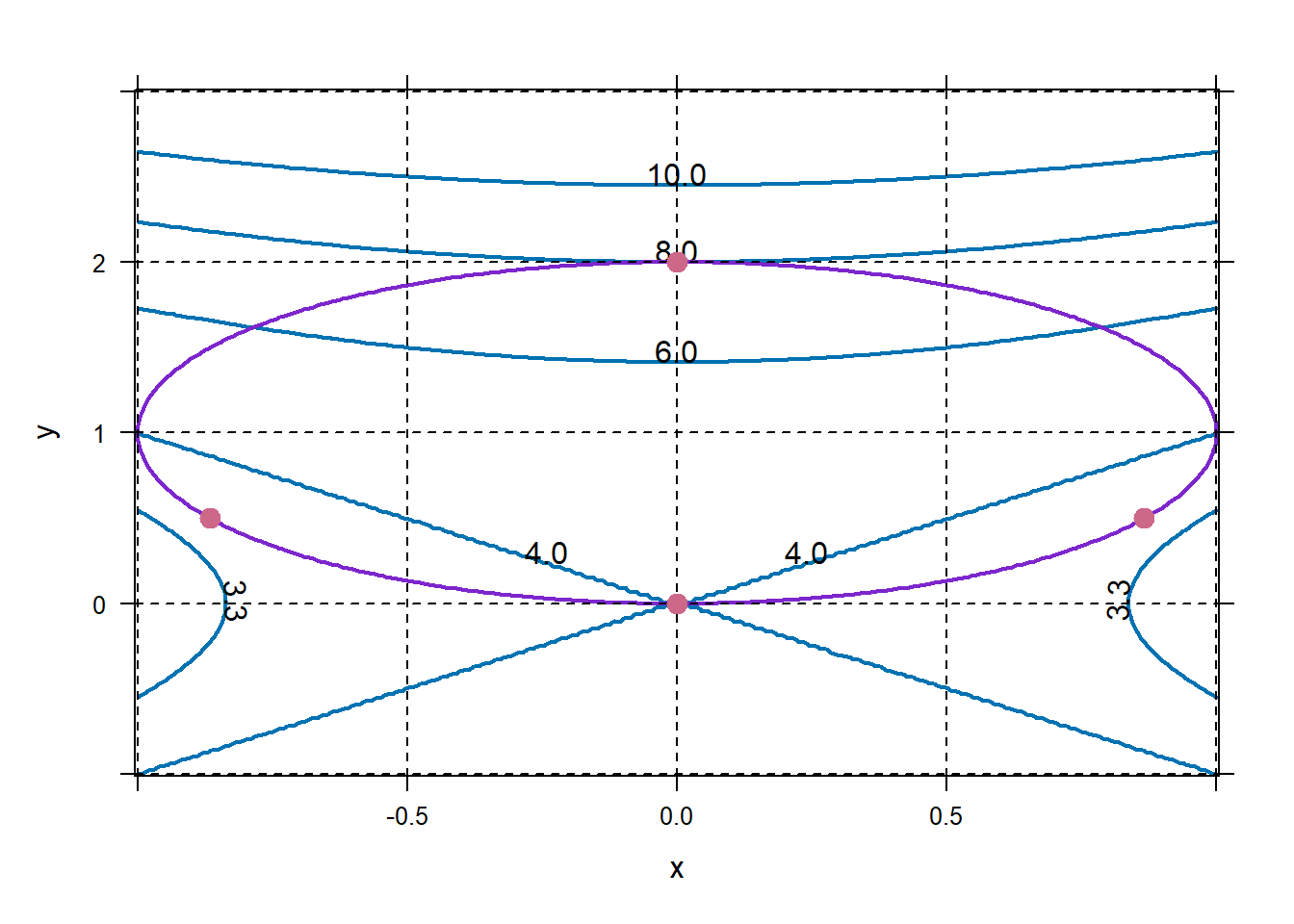

Great, we’ve got four possible extreme values. We can look at the figure above to figure out which ones are local mins and which ones are local maxes. Or, we can evaluate $f$.

c(f(-0.87,0.5),f(0,0),f(0,2),f(0.87,0.5))

## [1] 3.4931 4.0000 8.0000 3.4931

Example 7 is very nice. I’m going to modify it so that all components of the solution live in the range $\pm 100$. If you don’t want to modify the problem, use the option within to extend the range that findZeros looks in for the solution. Our objective function is $p(x,y)=200x^{3/4}y^{1/4}$. The modified constraint is $400x+200y=50000$.
```
p=makeFun(200*x^(3/4)*y^(1/4)~x&y)
Dpx=D(p(x,y)~x)
Dpy=D(p(x,y)~y)

g=makeFun(400*x+200*y~x&y)
Dgx=D(g(x,y)~x)
Dgy=D(g(x,y)~y)

cps=findZeros(c(Dpx(x,y) - l * Dgx(x,y), 
            Dpy(x,y) - l * Dgy(x,y), 
            g(x,y)-50000) ~x&y&l)
cps
```
```
##       x    y     l
## 1 93.75 62.5 0.339
```
Great, we have only one local extreme value, $(93.75,62.5)$, that results in a production of $p(93.75,62.5)=1.694254\times 10^{4}$. We can evaluate $p$ at other points that lie on our constraint, like $p(125,0)=0$, $p(0,250)=0$ to convince ourselves that we have found the maximum. The value of $\lambda$ tells us that for every extra dollar we add to the budget (from $50,000), we expect to produce an additional $0.34$ units.

If you want the unmodified constraint, do the following code, noting the within option.
```
p=makeFun(200*x^(3/4)*y^(1/4)~x&y)
Dpx=D(p(x,y)~x)
Dpy=D(p(x,y)~y)

g=makeFun(150*x+200*y~x&y)
Dgx=D(g(x,y)~x)
Dgy=D(g(x,y)~y)

cps=findZeros(c(Dpx(x,y) - l * Dgx(x,y), 
            Dpy(x,y) - l * Dgy(x,y), 
            g(x,y)-50000) ~x&y&l,within=1000)
cps
```
```
##     x    y     l
## 1 250 62.5 0.707
```
Exercises 50 – 56, Section 5.6. Avoid problem 57. findZeros will miss two of the solutions, even with the within option expanded. I’ve tried 50–56, they work fine.

2.9 Lesson 27: In-Class Project

2.9.1 Objectives

Given a real-world scenario, set up an appropriate multivariable optimization function and constraint equation.
Given an optimization function and constraint equation, use the method of Lagrange multipliers to find the location and/or value of the desired extrema subject to the constraint, by hand or using R.

2.9.2 In Class

Finish the In-Class project. Treat the handout as more-or-less a script. Go through the text with the students, have them complete the exercises, talk about the exercises.

2.9.3 R Commands

makeFun, fitModel, D, findZeros

Chapter 2 Block 2: Optimization

USAFACalc for Block 5

2.0.1 findZeros

2.0.1.1 Scalar equations

2.0.1.2 Options to help findZeros: near and within

2.0.2 Solving Systems of Equations with findZeros

2.0.3 Plotting functions of two variables, adding constraints

2.0.4 Plotting Vectors and Vector Fields

2.0.5 plotFun with surface option

2.1 Lesson 18: Extreme Values & Critical Numbers I

2.1.1 Objectives

2.1.2 Reading

2.1.3 In Class

2.1.4 R Commands

2.1.5 Problems & Activities

2.2 Lesson 19: Extreme Values and Critical Numbers II

2.2.1 Objectives

2.2.2 Reading

2.2.3 In Class

2.2.4 R Commands

2.2.5 Problems & Activities

2.3 Lesson 20: Concavity and Extreme Values

2.3.1 Objectives

2.3.2 Reading

2.3.3 In Class

2.3.4 R Commands

2.3.5 Problems & Activities

2.4 Lesson 21: Newton’s Method I

2.4.1 Objectives

2.4.2 Reading

2.4.3 In Class

2.4.4 R Commands

2.4.5 Problems & Activities

2.5 Lesson 22: Newton’s Method II

2.5.1 Objectives

2.5.2 Reading

2.5.3 In Class

2.5.4 R Commands

2.5.5 Problems & Activities

2.6 Lesson 23: Multivariable Optimization

2.6.1 Objectives

2.6.2 Reading

2.6.3 Special Notes

2.6.4 In Class

2.6.5 R Commands

2.6.6 Problems & Activities

2.7 Lesson 24: Constrained Optimization I

2.7.1 Objectives

2.7.2 Reading

2.7.3 In Class

2.7.4 R Commands

2.7.5 Problems & Activities

2.8 Lesson 25: Constrained Optimization II

2.8.1 Objectives

2.8.2 Reading

2.8.3 In Class

2.8.4 R Commands

2.9 Lesson 27: In-Class Project

2.9.1 Objectives

2.9.2 In Class

2.9.3 R Commands

`USAFACalc` for Block 5

2.0.1 `findZeros`

2.0.1.2 Options to help `findZeros`: `near` and `within`

2.0.2 Solving Systems of Equations with `findZeros`

2.0.5 `plotFun` with `surface` option