Chapter 11 Case study: Construction of the gene expression matrix for the raw data of the cohort GSE113179
In this case study, we will work with public data deposited on the Gene Expression Omnibus (GEO). We will cover all stages of the pipeline in order to demonstrate its application in real data. By the end of this study, you will be able to apply the pipeline to other public cohorts or to data generated by your laboratory.
11.1 Cohort contextualization
The cohort GSE113179 consists of four samples related to prostate cancer, being two controls and 2 knockout in the PC3 cell line. This cohort was deposited at GEO by Zhan Yang and Xiao-Lu Wang from 2018 to 2020 and is available at https://www.ncbi.nlm.nih.gov/geo/query/acc.cgi?acc=GSE113179.
11.2 Preparation of the work environment
We could generate the scripts and directory structure without having to download the repository. But to make the most of the time, we’ll use the scripts and directories in the repository and change them as needed.
11.3 Directory structure and scripts
Let’s download the PreProcSEQ repository and set it as a working environment:
cd ~
wget https://github.com/resendejss/PreProcSEQ/archive/refs/heads/main.zip
unzip main.zip
cd ~/PreProcSEQ-main
Let’s delete the sample samples from the 0-samples directory:
rm 0-samplees/*11.4 Installation of tools
We could install one tool at a time, or research the best way to install it, however, the pipeline already has a script that installs the tools. Let’s run the installTools.sh bash script to install the necessary tools:
./installTools.sh11.5 Obtaining samples
There are a few ways to get GEO samples, feel free to choose your preferred method. We will use WGET to access the FTP links for each sample.
Let’s build the bash script to download the samples. Use your favorite text editor and save the following commands in a sh file (downloadSamples.sh) in the working directory (PreProcSEQ-main):
#!/bin/bash

cd ~/PreProcSEQ-main/0-samples

wget ftp://ftp.sra.ebi.ac.uk/vol1/fastq/SRR700/002/SRR7009362/SRR7009362_1.fastq.gz
wget ftp://ftp.sra.ebi.ac.uk/vol1/fastq/SRR700/002/SRR7009362/SRR7009362_2.fastq.gz
wget ftp://ftp.sra.ebi.ac.uk/vol1/fastq/SRR700/003/SRR7009363/SRR7009363_1.fastq.gz
wget ftp://ftp.sra.ebi.ac.uk/vol1/fastq/SRR700/003/SRR7009363/SRR7009363_2.fastq.gz
wget ftp://ftp.sra.ebi.ac.uk/vol1/fastq/SRR700/004/SRR7009364/SRR7009364_1.fastq.gz
wget ftp://ftp.sra.ebi.ac.uk/vol1/fastq/SRR700/004/SRR7009364/SRR7009364_2.fastq.gz
wget ftp://ftp.sra.ebi.ac.uk/vol1/fastq/SRR700/005/SRR7009365/SRR7009365_1.fastq.gz
wget ftp://ftp.sra.ebi.ac.uk/vol1/fastq/SRR700/005/SRR7009365/SRR7009365_2.fastq.gz
Convert the script into an executable:
chmod +x downloadSamples.shThen run the script in the terminal:
./downloadSamples.sh11.6 Quality control
With the samples in the 0-samples directory, we will run the qualityControl_beforeTrimming.sh script in order to get the quality control results of the samples.
Before running the script, let’s check if you need to change any variables in the script:
cat qualityControl_beforeTrimming.shThere is no need to change any variables, as FastQC will access the 0-samples samples and analyze them. The result for each sample will be stored in 1-qualityControl_beforeTrimming/outputFastqc. MultiQC will group the FastQC outputs and store that result in 1-qualityControl_beforeTrimming/outputMultiqc.
Below is the first FastQC result with MultiQC: General Statistics. The first column contains the name of the samples. The second column represents the content of duplicate reads. The third column shows the GC content and finally, in the fourth column, the number of readings is in millions (M).
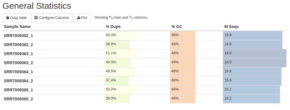 This table presents the main statistical results. We will see these results further in the graphs below. But this table shows us that there are read duplications - which is expected in RNA-Seq data. The GC content is close to what is expected for human data (can vary from 35 to 60% in 100 kb data with an average of 41%). Finally, the number of readings per sample.
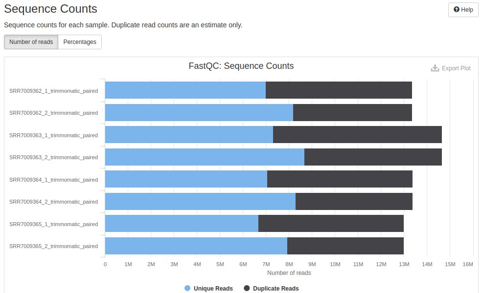
Then, a horizontal bar graph is presented representing the amount of duplicate readings and unique readings for each sample, further detailing the data presented in the second column of the table presented above.

The next metric evaluated was the average quality of the sequenced bases. The background colors indicate whether the average for a given position was bad (red), acceptable (yellow) and good (green). Each line within the graph represents a file. The X and Y axes represent the position of each nucleotide and the quality score, respectively.
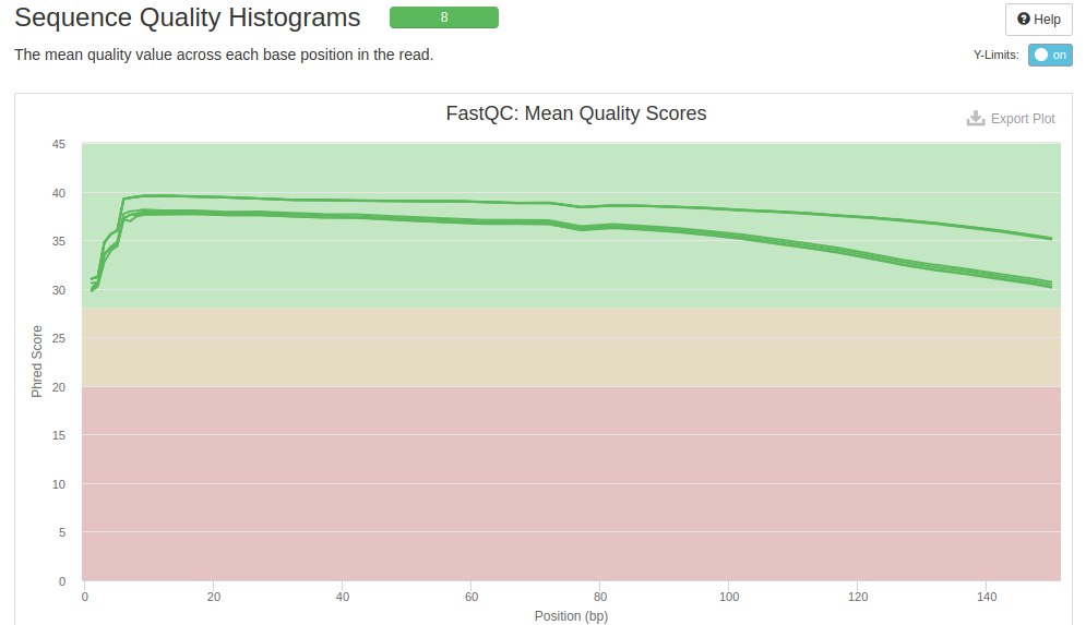
It is seen that all analyzed files (six files) had very good quality score averages. But there is a drop in quality at the beginning and end of the reads - which is also expected in Illumina sequencers.
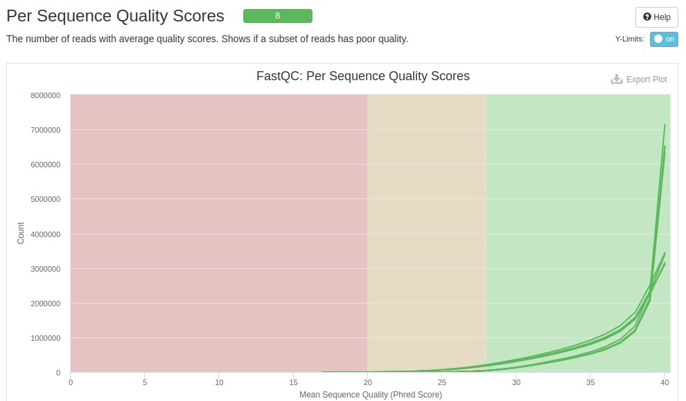
The next graph shows the quality score on the X axis and the amount of reads on the Y axis. Each line within the graph represents a file and the background colors represent bad (red), acceptable (yellow) and good (green).
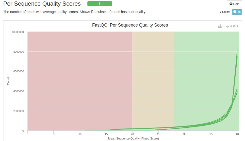
It is seen that most of the readings were in the green region, and with a higher concentration close to 40. However, it is noted that there are some readings with low quality scores (score < 20 - red region).
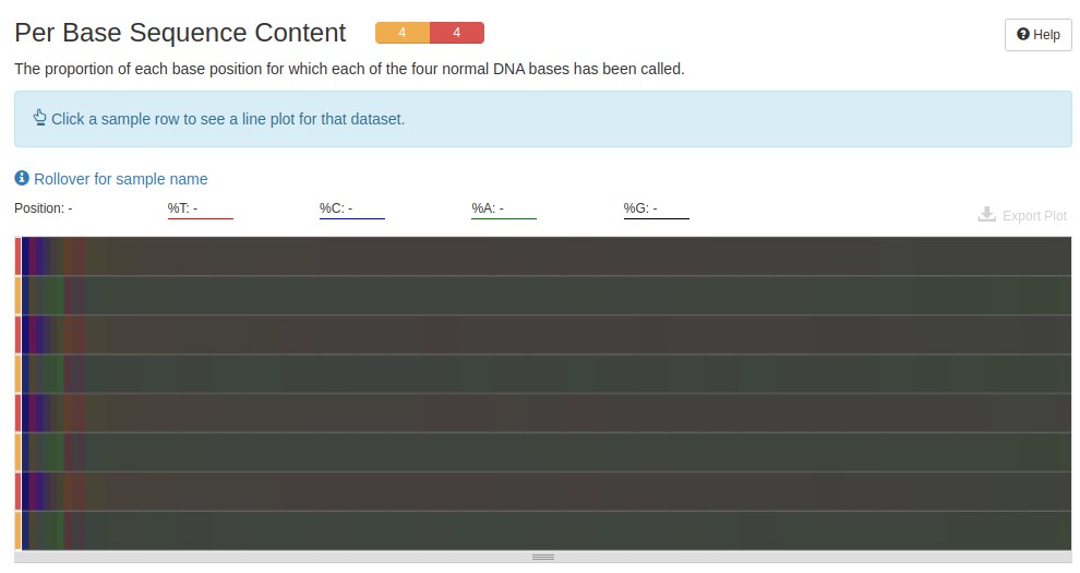
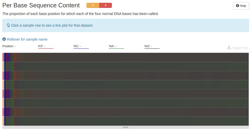
The next graph shows the amount of A, C, T and G in each file. In data produced by RNA-Seq, it is normal to find at the beginning of the readings a base pair mismatch, that is, C-G and A-T.
The next graph shows the GC content. The lines represent the files and their coloring indicates whether it is good (green) or acceptable (yellow). If it had red it would be the fault. But in RNA-seq, the GC content may change due to transcript expression, however, it is necessary to pay attention if there is contamination of another organism in the samples.

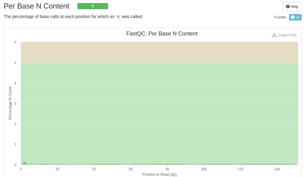
The N content plot shows the bases that were not identified by the sequencer. Each line represents a file. The background color indicates whether or not the file needs repair when compared to unidentified bases.
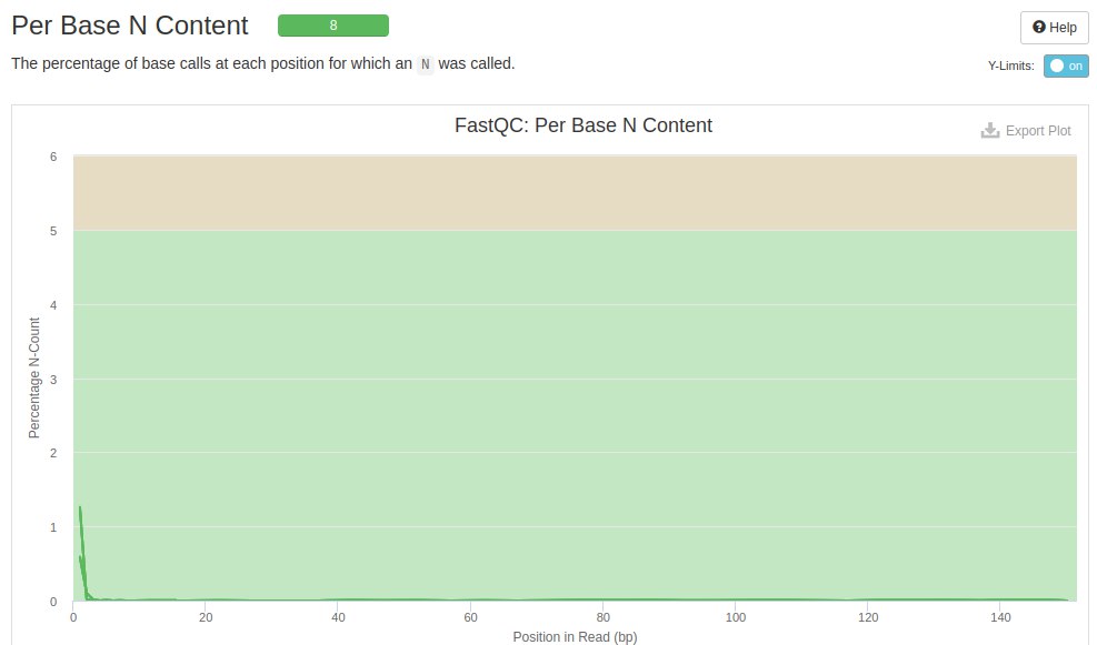
In these samples it is seen that at the beginning of the readings some bases were not identified. According to FastQC these bases will not interfere with further analysis as it has not exceeded the 5% limit.
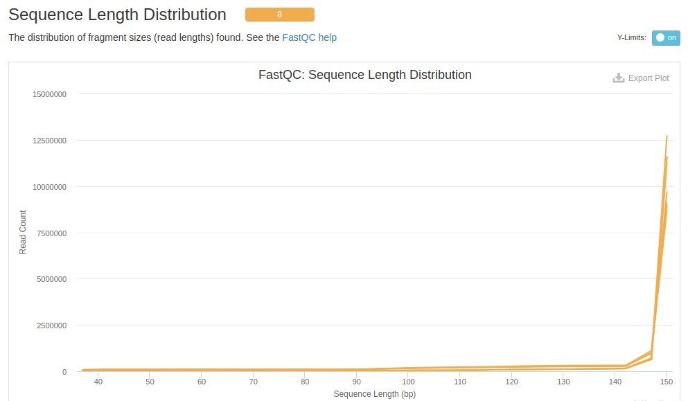
The next evaluation is about the length of the readings, in this case the readings are 150 bp.

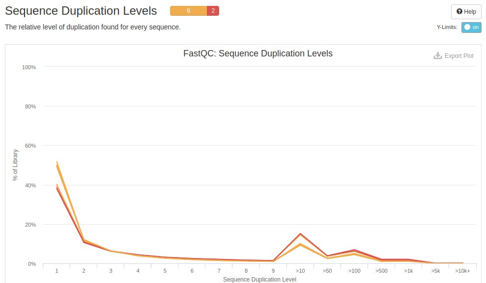
The next chart is about duplicate readings. In RNA-seq data it is common and expected to find duplications. FastQC is not designed for expression data, but for genomic data, so it classifies duplicates as failures.
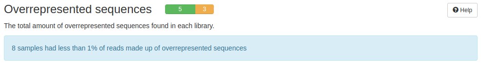
Another analysis that FastQC did was the evaluation of overrepresented sequences. Depending on the construction of the cDNA library, as well as the handling of the samples, FastQC can identify sequences that are over-represented and fault them. But in RNA-seq data, there are sequences/reads that are highly represented. This result depending on the project can be a bias or can be a biological result.
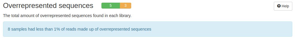
In this case the files went through QC, but there are cases where the adapter sequence appears as super represents and this can result in changes in the alignment or mapping of the readings.
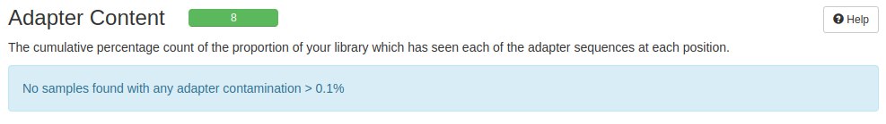
The next graph presents the adapters found in the analyzed files. Each row represents an adapter type. The background color as in the previous graphics represents acceptance of the files as they are.

In this case, some sequences that match adapters were found. Some adapter readings are complete, but the greatest concentration is at the end of the readings. According to FastQC, there are a number of adapters that can interfere with subsequent analyses.
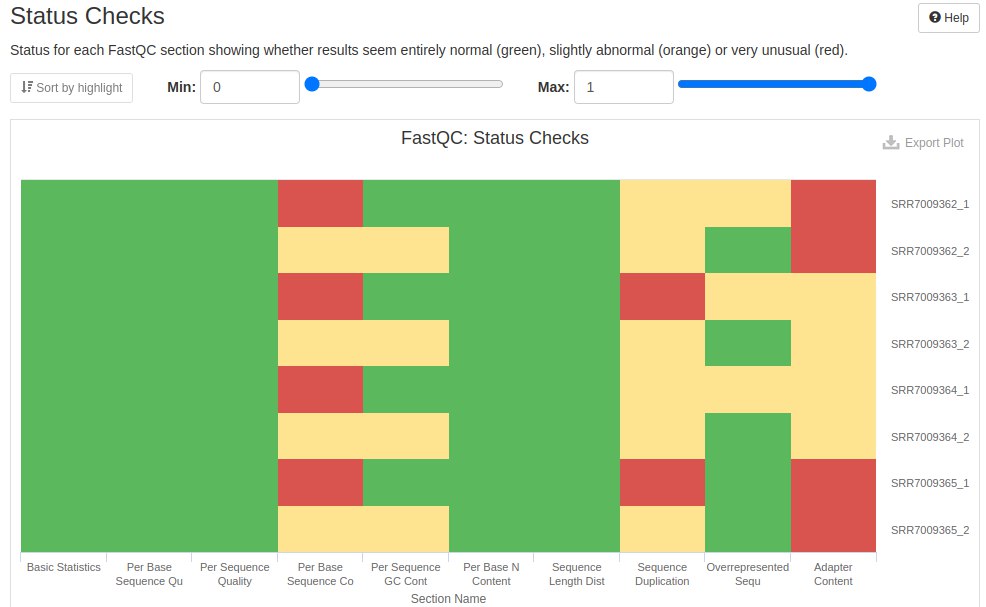
Finally, a summary of the evaluated metrics is presented. What passed the QC is marked green and what did not pass is colored red. What was acceptable, but needs attention, was left with yellow.
11.7 Trimming
After evaluating the QC of the raw data, we will trim the readings. According to the pipeline, we will use the Trimmomatic tool to filter the readings and remove the adapter sequences.
The pipeline provides the script to run Trimmomatic (trimming_trimmomatic.sh). Let’s change it as per our samples:
cat ~/PreProcSEQ-main/trimming_trimmomatic.sh## #!/bin/bash
## INPUT="0-samples"
## OUTPUTP="2-trimming/trimmomatic/paired"
## OUTPUTUNP="2-trimming/trimmomatic/unpaired"
##
## time while read SAMP \n
## do
## TrimmomaticPE $INPUT/${SAMP}_R1.fastq $INPUT/${SAMP}_R2.fastq \
## $OUTPUTP/${SAMP}_R1_trimmomatic_paired.fastq \
## $OUTPUTUNP/${SAMP}_R1_trimmomatic_unpaired.fastq \
## $OUTPUTP/${SAMP}_R2_trimmomatic_paired.fastq \
## $OUTPUTUNP/${SAMP}_R2_trimmomatic_unpaired.fastq \
## ILLUMINACLIP:TruSeq3-PE-2.fa:2:30:10 \
## LEADING:3 TRAILING:3 SLIDINGWINDOW:4:15 MINLEN:36
## done < samplesNames.txtFirst let’s build the samplesNames.txt file with the names of the samples we are working on:
dir <- "~/PreProcSEQ-main/0-samples/"
files <- list.files(paste0(dir))
samples_names <- unique(gsub("_..fastq.gz","",files))
write.table(samples_names,"~/PreProcSEQ-main/samplesNames.txt",
            quote = F, row.names = F, col.names = F)
Next, let’s change the sample names’ complement to $INPUT and $OUTPUT in the script:
#!/bin/bash
INPUT="0-samples"
OUTPUTP="2-trimming/trimmomatic/paired"
OUTPUTUNP="2-trimming/trimmomatic/unpaired"

time while read SAMP \n
            do
            TrimmomaticPE $INPUT/${SAMP}_1.fastq.gz $INPUT/${SAMP}_2.fastq.gz \
            $OUTPUTP/${SAMP}_1_trimmomatic_paired.fastq.gz \
            $OUTPUTUNP/${SAMP}_R1_trimmomatic_unpaired.fastq.gz \
            $OUTPUTP/${SAMP}_2_trimmomatic_paired.fastq.gz \
            $OUTPUTUNP/${SAMP}_2_trimmomatic_unpaired.fastq.gz \
            ILLUMINACLIP:TruSeq3-PE-2.fa:2:30:10 \
            LEADING:3 TRAILING:3 SLIDINGWINDOW:4:15 MINLEN:36
        done < samplesNames.txt
Then run the script in the terminal:
./trimming_trimmomatic.shThe processed samples will be saved in 2-trimming/trimmomatic. In the paired directory will be the filtered samples. In the unpaired directory will be the readings taken from the samples.
11.8 Quality control after trimming
Let’s verify that the trimming step has removed the low quality bases and adapter sequences. For this we will run the qualityControl_afterTrimmomatic.sh script. But first let’s check if the variables and names of the ones agree with our samples:
cat ~/PreProcSEQ-main/qualityControl_afterTrimming.sh## #!/bin/bash
## INPUTFASTQC="2-trimming/trimmomatic/paired"
## OUTPUTFASTQC="3-qualityControl_afterTrimming/outputFastqc"
## OUTPUTMULTIQC="3-qualityControl_afterTrimming/outputMultiqc"
##
## /usr/bin/time -f "\nResultado do time: \nTempo decorrido = %E" \
## fastqc $INPUTFASTQC/* -o $OUTPUTFASTQC
##
## /usr/bin/time -f "\nResultado do time: \nTempo decorrido = %E" \
## multiqc $OUTPUTFASTQC/. -o $OUTPUTMULTIQCWe won’t need to change anything in the script. So let’s run it in the terminal:
./qualityControl_afterTrimmomatic.shOverall statistics show that there were some differences in duplications and GC content between the data before and after trimming. These differences were in response to the third column - M Seqs - the amount of reads. Before trimming there were 16.8, 18.0, 16.6 and 16.2 for R1 and R2. After trimming, the amount of readings for R1 and R2 went to 13.4, 14.6, 13.4 and 13.0. That is, the trimming step removed some readings.
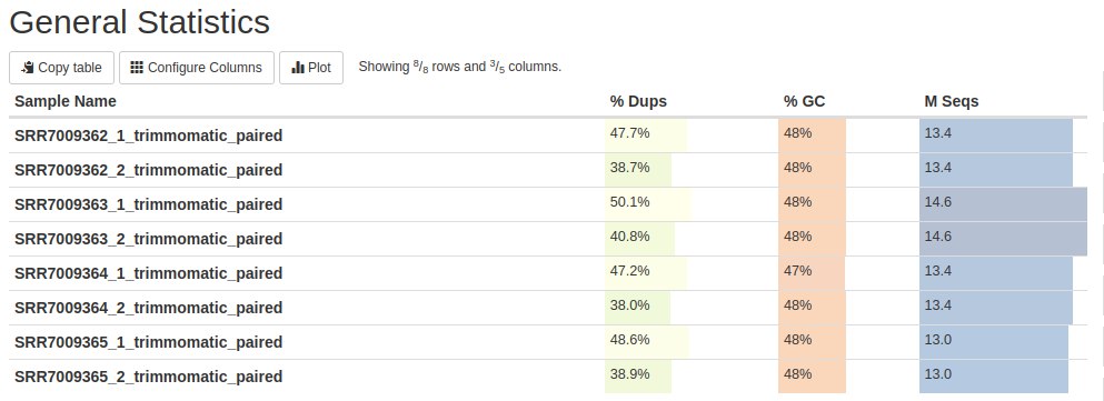 The duplications remained with the same profile: R1 with more duplications than R2. But there was a difference in the number of readings, as seen earlier.
 The averages of the quality scores showed that the bad readings were removed. There was a big improvement at the end of the reads, indicating that if the adapter sequences were removed, they were causing more of this quality drop.

When analyzing the quality score per read, it is seen that the trimming step removed the reads with scores below 17. This explains some of the improvement in the files in the previous figure and the differences in the amounts of reads before and after trimming.
The content profile of the bases before trimming proved to be very similar to this profile after trimming. To better visualize the differences, I would need to interact with the mouse in the desired positions and see the difference from one profile to the other.
 As for the GC content, the results were similar, to find the difference between the graphics, you would need to use the cursor and interact with the image and check the points.

The graph below shows that the trimming removed the unidentified bases at the beginning of the readings. This removal contributed to the improvement in the quality of the data.
After trimming, the lengths of the readings were between 37 to 150 bp, with a higher concentration between 140 to 150 bp. This showed that in addition to the Trimmomatic removing some readings, it also pb and kept the readings of those pb.
The next graph shows the levels of sample duplications. Some regions had higher expressions - which is also expected in RNA-Seq, unlike genomic data.

FastQC did not identify overrepresented sequences. That is, there are duplicate readings but not in an exaggerated way.
The trimming step removed the adapters that FastQC had identified.
 Finally, the status of each evaluation performed by FastQC is presented, informing which metrics were evaluated and which samples passed. Remembering that FastQC was not developed specifically for eexpression data, so some metrics are disregarded.

11.9 Quantification
Let’s move on to the quantification of the transcripts with the trimmed data, that is, with the files processed by Trimmomatic (2-trimming/trimmomatic/paired).
The pipeline provides two tools for the quantification of transcripts: Kallisto and Salmon. We will use Salmon, because it is a more current tool and has some parameters to correct some biases.
11.9.1 Obtaining the reference transcriptome
The pipeline includes the GENCODE v.40 reference transcriptome, but if you prefer, you can download the transcriptome as follows:
setwd("~/PreProcSEQ-main")
transcriptome_file <- "ftp://ftp.ebi.ac.uk/pub/databases/gencode/Gencode_human/release_40/gencode.v40.transcripts.fa.gz"
download.file(transcriptome_file,"gencode.v40.transcripts.fa.gz")
If you want to use another version of the transcriptome or the latest one, change v40 to the desired version.
11.9.2 Building the transcriptome index
Salmon like Kallisto needs a reference transcriptome index. The pipeline brings the pre-built script for this build (salmon_index.sh), let’s preview it to see if it needs to change any parameters:
cat ~/PreProcSEQ-main/salmon_index.sh## #!/bin/bash
##
## time salmon index -t gencode.v40.transcripts.fa.gz \
## -i 4-quantification/salmon/gencode_v40_indexIf we are going to work with the v40 transcriptome we won’t need to change anything in the script, but if you chose to download another version, change the name gencode.v40.transcripts.fa.gz to the name of the transcriptome you downloaded.
Let’s run the salmon_index.sh script:
./salmon_index.sh11.9.3 Quantification of transcripts
After building the reference transcriptome index, we can quantify the transcripts. Before running the script, let’s see in the script what we need to change to read our files (salmon_quant.sh):
cat ~/PreProcSEQ-main/salmon_quant.sh## #!/bin/bash
##
## time while read SAMP \n
## do
## echo "Processing sample ${SAMP}"
## salmon quant -i 4-quantification/salmon/gencode_v40_index -l A \
## -1 2-trimming/trimmomatic/paired/${SAMP}_R1_trimmomatic_paired.fastq \
## -2 2-trimming/trimmomatic/paired/${SAMP}_R2_trimmomatic_paired.fastq \
## -p 4 --gcBias --validateMappings -o 4-quantification/salmon/quant_salmon/${SAMP}_quant
## done < samplesNames.txtThe samplesNames we already have, we will need to change the argument extension -1 and -2:
#!/bin/bash

time while read SAMP \n
        do
            echo "Processing sample ${SAMP}"
            salmon quant -i 4-quantification/salmon/gencode_v40_index -l A \
            -1 2-trimming/trimmomatic/paired/${SAMP}_1_trimmomatic_paired.fastq.gz \
            -2 2-trimming/trimmomatic/paired/${SAMP}_2_trimmomatic_paired.fastq.gz \
            -p 4 --gcBias --validateMappings -o 4-quantification/salmon/quant_salmon/${SAMP}_quant
        done < samplesNames.txt
After making the changes, let’s run the script:
./salmon_quant.shThe quantifications will be saved in 4-quantification/salmon/quant_salmon. Four directories will be generated, referring to the four samples. Each directory will contain some files, among them quant.sf is the file that contains the quantifications.
ls ~/PreProcSEQ-main/4-quantification/salmon/quant_salmon/SRR7009362_quant## aux_info
## cmd_info.json
## lib_format_counts.json
## libParams
## logs
## quant.sf11.10 Construction of the gene expression matrix
Salmon quantified the transcripts for each sample. Now it is necessary to build the gene expression matrix with the data with the quant.sf files of each sample, which contain the transcript quantifications in TPM, raw counts and transcript length.
We will use the R/Bioconductor package tximeta to import the files and summarize them in matrices, as well as join them with the metadata of the samples and the transcripts. But first let’s build the metadata of the samples according to the information in the cohort repository.
# -- metadados das amostras
coldata <- data.frame(
  id = c("SRR7009362","SRR7009363","SRR7009364","SRR7009365"),
  title = c("con-1","con-2","p53-1","p53-2"),
  cell_linee = rep("PC3",4),
  gender = rep("male",4)
)

DT::datatable(coldata)
The pipeline provides the script in R for building the matrix with the quantifications generated by Salmon (matrixConstruction_tximeta_salmon.R). Let’s open the script and change whatever is necessary.
library(tximeta)
library(SummarizedExperiment)
#library(readxl) # nao vai precisar
library(GenomicFeatures)

setwd("~/PreProcSEQ-main/5-expressionMatrix/tximeta")
dirquant <- "~/PreProcSEQ-main/4-quantification/salmon/quant_salmon/"

#coldata <- read_xlsx("../../metadata.xlsx") ## eesse dado reefere-se as amostras deed exemplo
coldata$names <- coldata$id # troque o 'Sample_id' por 'id'
coldata$files <- paste0(dirquant,coldata$names,"_quant/","quant.sf")
all(file.exists(coldata$files))
coldata <- as.data.frame(coldata)
rownames(coldata) <- coldata$names

indexDir <- file.path("../../4-quantification/salmon/gencode_v40_index")
gffPath <- file.path("../../gencode.v40.annotation.gff3.gz")
fastaFTP <- "ftp.ebi.ac.uk/pub/databases/gencode/Gencode_human/release_40/gencode.v40.transcripts.fa.gz"

makeLinkedTxome(indexDir = indexDir,
                source = "GENCODE",
                organism = "Homo sapiens",
                release = "40",
                genome = "GRCh38",
                fasta = fastaFTP,
                gtf = gffPath,
                write = FALSE)

se <- tximeta(coldata, useHub = F)
gse <- summarizeToGene(se)

save(gse, file="matrix_gse_salmon_tximeta.RData")
After running the commands, the gse object which contains the matrix information will be saved in 5-expressionMatrix/tximeta.
In gse@colData you have the metadata of the samples and in gse@rowranges you have the metadata of the transcripts. As for arrays, they are in gse@assays@data. In gse@assays@data$counts are the raw counts, gse@assays@data$abundance are the normalized counts in TPM and `gse@assays@data$length are the lengths of the transcripts.
Let’s view the raw counts, TPM counts, and transcript lengths for the first five transcripts and for all samples:
load("~/PreProcSEQ-main/5-expressionMatrix/tximeta/matrix_gse_salmon_tximeta.RData")
DT::datatable(gse@assays@data$counts[1:5,])
## Loading required package: S4Vectors## Loading required package: stats4## Loading required package: BiocGenerics##
## Attaching package: 'BiocGenerics'## The following objects are masked from 'package:stats':
##
## IQR, mad, sd, var, xtabs## The following objects are masked from 'package:base':
##
## anyDuplicated, aperm, append, as.data.frame, basename, cbind,
## colnames, dirname, do.call, duplicated, eval, evalq, Filter, Find,
## get, grep, grepl, intersect, is.unsorted, lapply, Map, mapply,
## match, mget, order, paste, pmax, pmax.int, pmin, pmin.int,
## Position, rank, rbind, Reduce, rownames, sapply, setdiff, sort,
## table, tapply, union, unique, unsplit, which.max, which.min##
## Attaching package: 'S4Vectors'## The following objects are masked from 'package:base':
##
## expand.grid, I, unnameDT::datatable(gse@assays@data$abundance[1:5,])DT::datatable(gse@assays@data$length[1:5,])11.11 Annotation of transcripts
Let’s put more information from the transcripts in the gse object. For this, we will also use the script provided by the pipeline (annotationTranscripts_salmon_matrixTximeta.R). We won’t need to change anything in the script, and the annotated object will be saved in 6-annotationTranscripts:
library(AnnotationHub)
library(GenomicFeatures)
library(ensembldb)
library(SummarizedExperiment)

setwd("~/PreProcSEQ-main/6-annotationTranscripts")

ah <- AnnotationHub()

edb <- query(ah, pattern = c("Homo sapiens", "EnsDb",106))[[1]]
gns <- genes(edb)
EnsDbAnnotation <- as.data.frame(gns)
EnsDbAnnotation <- EnsDbAnnotation[,c("gene_id","symbol","gene_biotype","entrezid")]
dim(EnsDbAnnotation)
colnames(EnsDbAnnotation) <- c("ensemblid","symbol","gene_biotype","entrezid")

load("../5-expressionMatrix/tximeta/matrix_gse_salmon_tximeta.RData")

nrow(gse)
gseAnnotation <- rowData(gse)

rownames(gseAnnotation) <- stringr::str_replace(rownames(gseAnnotation), "\\...$", "")
rownames(gseAnnotation) <- stringr::str_replace(rownames(gseAnnotation), "\\..$", "")

all(rownames(gseAnnotation)%in%rownames(EnsDbAnnotation))

rowAnnotation <- EnsDbAnnotation[rownames(gseAnnotation),]
rowAnnotation <- data.frame(gseAnnotation, rowAnnotation, stringsAsFactors = F)
rownames(rowAnnotation) <- rowAnnotation$gene_id
rowData(gse) <- rowAnnotation

save(gse, file = "matrix_gse_salmon_tximeta_noted.RData")
11.12 Normalization of counts
Salmon generates the quantifications in raw counts and normalized in TPM. Depending on the analysis, a raw count is necessary, and for others, normalized counts are more interesting, due to some biases such as the size of the transcript and the cDNA library.
In the gse object we have the raw counts (gse@assays@data$counts) and the normalized counts in TPM (gse@assays@data$abundance). Let’s replace TPM normalization with TMM. For this, we will use the script provided by the pipeline - normalizationTMM.R:
library(edgeR)
library(SummarizedExperiment)

setwd("~/PreProcSEQ-main/7-normalizationCounts/tmm/")
load("../../6-annotationTranscripts/matrix_gse_salmon_tximeta_noted.RData")

gexp.counts.brut <- assay(gse)

dge <- DGEList(counts=gexp.counts.brut)
dge <- calcNormFactors(dge)
gexp.TMM <- cpm(dge)

gse.TMM <- gse
gse.TMM@assays@data$abundance <- gexp.TMM
save(gse.TMM, file = "gse_tmm.RData")
The normalized counts in TMM are in gse@assays@data$abundance in the gse object in the 7-normalizationCounts/tmm directory.