Exercise Solutions

Section 1.1.1

You should expect these variables to be very closely correlated, with the points clustered very close to a line.

ggplot(data = mpg) +
  geom_point(mapping = aes(x = cty, y = hwy))

manufacturer, model, year, cyl, trans, drv, fl, and class are categorical. The others are continuous. (You could make an argument for year and cyl being continuous as well, but because each only has a few values and the possible values cannot occur across a continuous spectrum, they are more appropriately classified as categorical.)
You could use either hwy or cty to measure fuel efficiency. The scatter plot below would indicate that front-wheel drives generally have the best fuel efficiency but exhibit the most variation. Rear-wheel drives get the worst fuel efficiency and exhibit the least variation.

ggplot(data = mpg) +
  geom_point(mapping = aes(x = drv, y = hwy))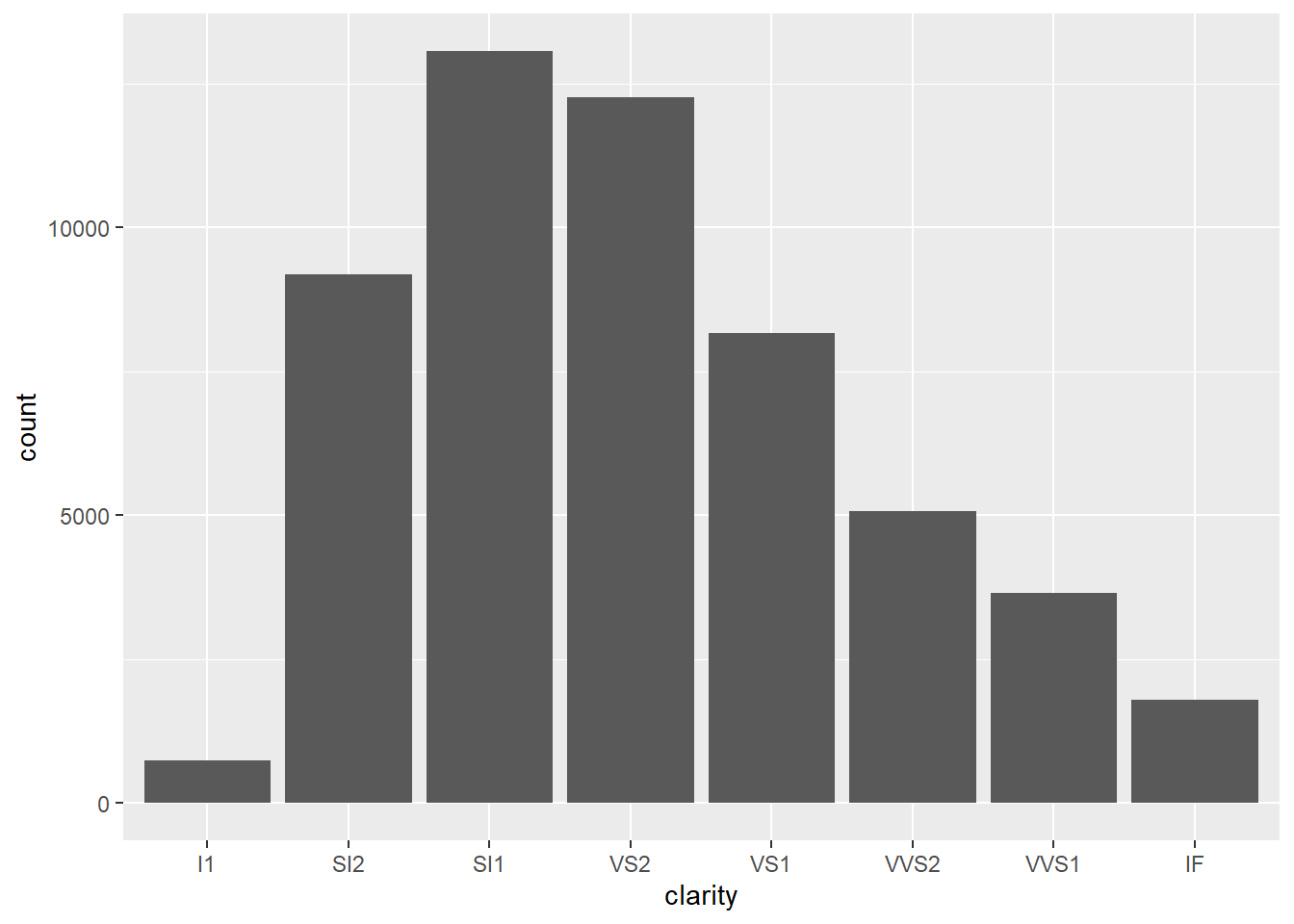

The points are stacked vertically. This happens because drv is categorical. (We’ll see in Section 1.6 that box plots are better ways to visualize a continuous vs. categorical relationship.)
In the scatter plot below, a dot just indicates that a car with that class-drv combination exists in the data set. For example, there’s a car with class = 2seater and drv = r. While this is somewhat helpful, it doesn’t convey a trend, which is what scatter plots are supposed to do.

ggplot(data = mpg) +
  geom_point(mapping = aes(x = class, y = drv))

Scatter plots are most useful when they illustrate a trend in the data, i.e., a way that a change in one variable brings about a change in a related variable. Changes in variables are easier to think about and visualize when the variables are continuous.

Section 1.2.1

The warning message indicates that you can only map a variable to shape if it has 6 or fewer values since looking at more than 6 shapes can be visually confusing. The 62 rows that were removed must be those for which class = SUV since SUV is the seventh value of class when listed alphabetically.

ggplot(data = mpg) +
  geom_point(mapping = aes(x = displ, y = hwy, shape = class))

## Warning: The shape palette can deal with a maximum of 6 discrete values because more than 6 becomes
## difficult to discriminate; you have 7. Consider specifying shapes manually if you must have
## them.

## Warning: Removed 62 rows containing missing values (geom_point).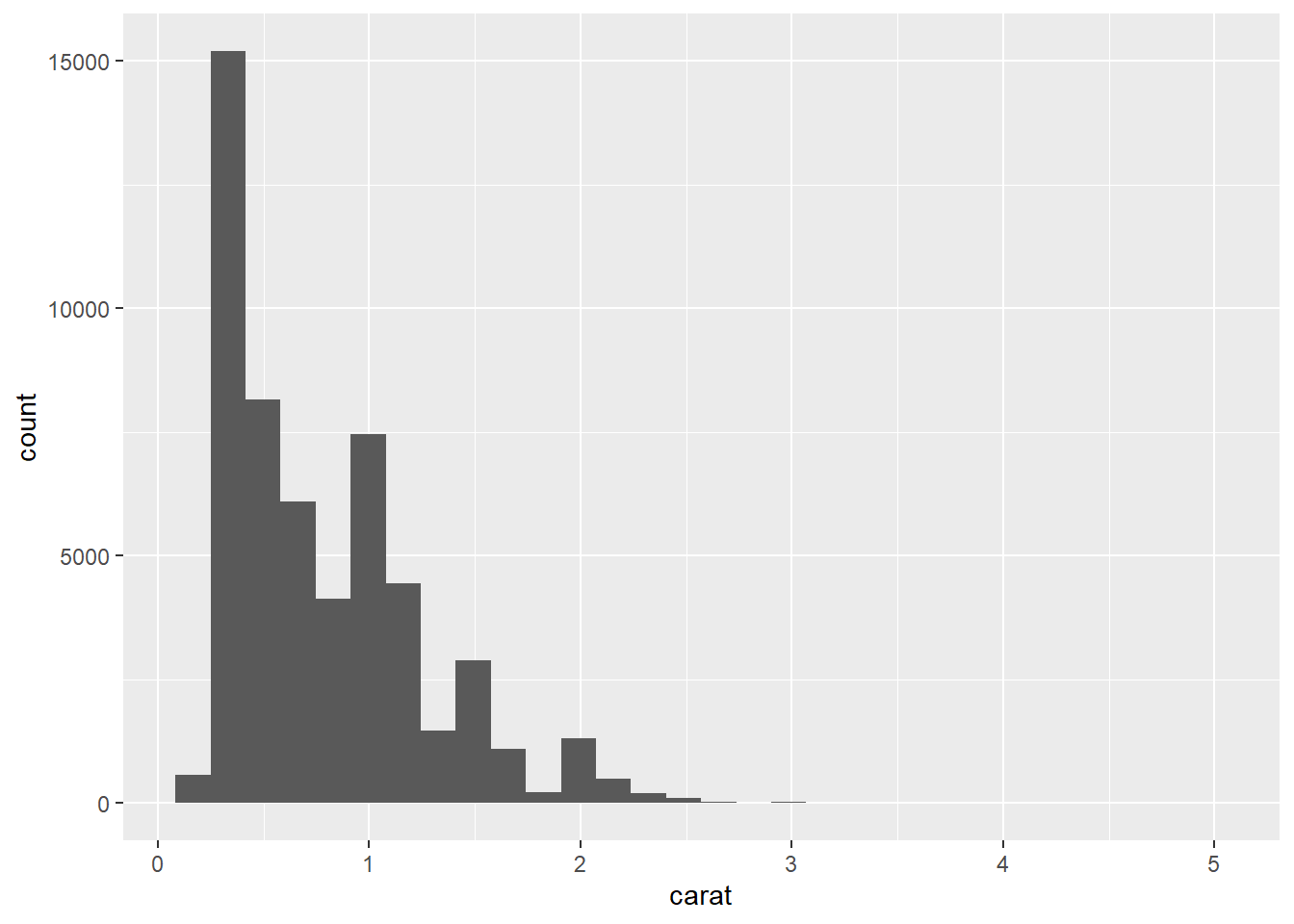

One example would be to use drv instead of class since it only has 3 values:

ggplot(data = mpg) +
  geom_point(mapping = aes(x = displ, y = hwy, shape = drv))

The scatter plot below shows what happens when the continuous variable cty is mapped to shape. The error message indicates that this is not an option.

ggplot(data = mpg) +
  geom_point(mapping = aes(x = displ, y = hwy, shape = cty))

## Error in `scale_f()`:
## ! A continuous variable can not be mapped to shape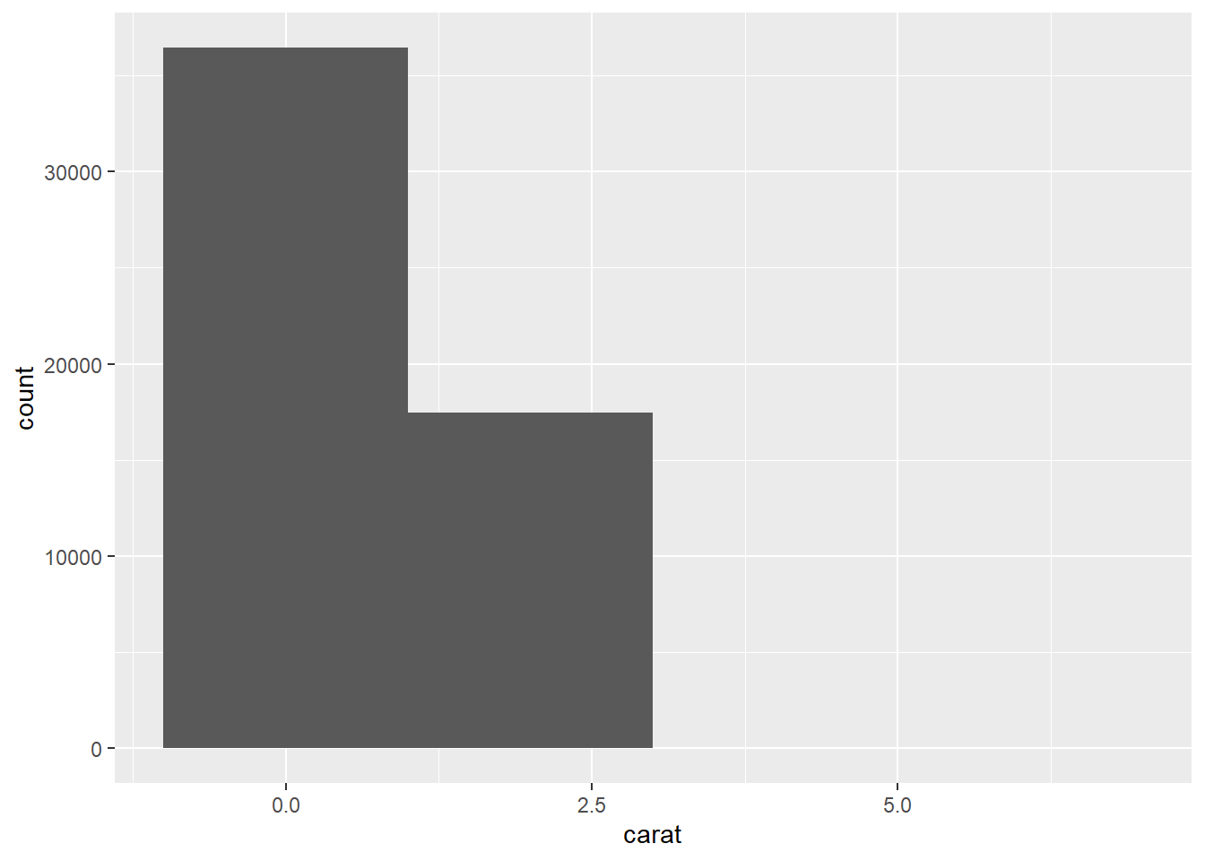

First, let’s map the continuous cty to size. We see that the size of the dots corresponds to the magnitude of the values of cty. The legend displays representative dot sizes.

ggplot(data = mpg) +
  geom_point(mapping = aes(x = displ, y = hwy, size = cty))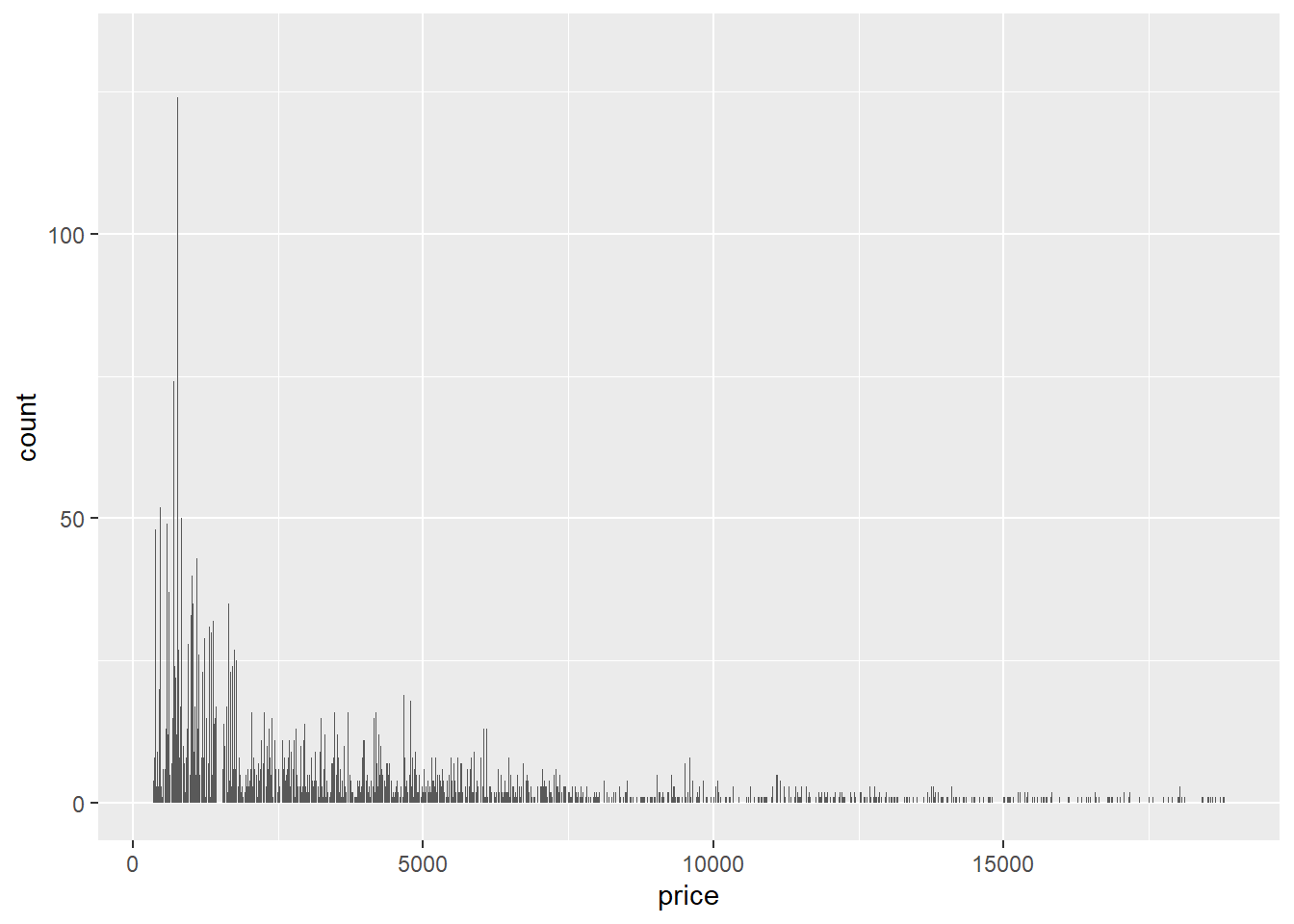

If we map the categorical drv to size, we get a warning message that indicates that size is not an appropriate aesthetic for categorical variables. This is because such variables usually have no meaningful notion of magnitude, so the size aesthetic can be misleading. For example, in the plot below, one might get the idea that rear-wheel drives are somehow “bigger” than front-wheel and 4-wheel drives.

ggplot(data = mpg) +
  geom_point(mapping = aes(x = displ, y = hwy, size = drv))

## Warning: Using size for a discrete variable is not advised.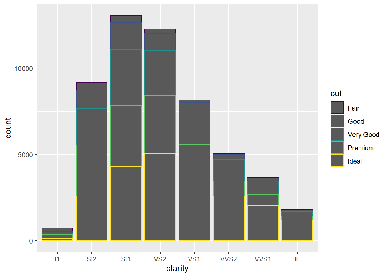

Mapping the continuous cty to color, we see that a gradation of colors is assigned to the continuous interval of cty values.

ggplot(data = mpg) +
  geom_point(mapping = aes(x = displ, y = hwy, color = cty))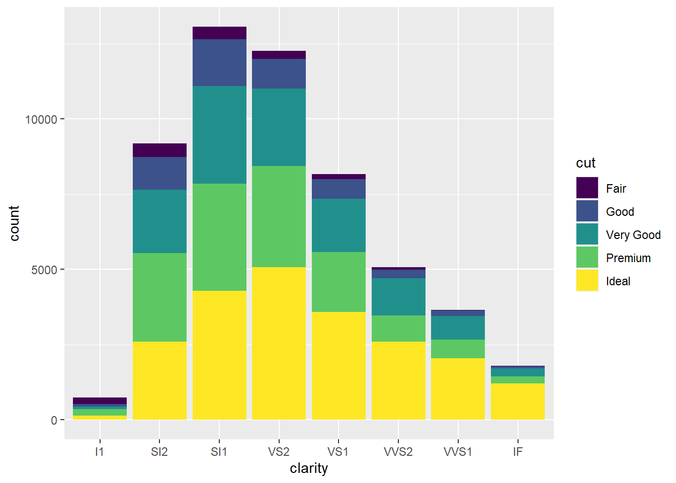

The scatter plot below maps class to color and drv to shape. The result is a visualization which is somewhat hard to read. Generally speaking, mapping to more than one extra aesthetic crams a little too much information into a visualization.

ggplot(data = mpg) +
  geom_point(mapping = aes(x = displ, y = hwy, color = class, shape = drv))

The scatter plot below maps the drv variable to both color and shape. Mapping drv to two different aesthetics is a good way to further differentiate the scatter plot points that represent the different drv values.

ggplot(data = mpg) +
  geom_point(mapping = aes(x = displ, y = hwy, color = drv, shape = drv))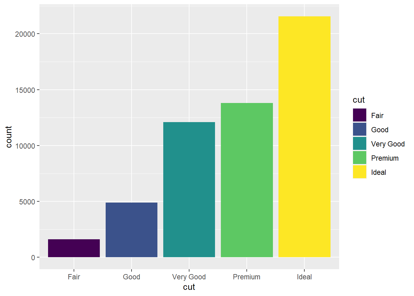

This technique gives us a way to visually separate a scatter plot according to a given condition. Below, we can visualize the relationship between displ and hwy separately for cars with fewer than 6 cylinders and those with 6 or more cylinders.

ggplot(mpg) +
  geom_point(aes(displ, hwy, color = cyl<6))

Section 1.4.1

The available aesthetics are found in the documentation by entering ?geom_smooth. The visualizations below map drv to linetype and size.

ggplot(data = mpg) +
  geom_smooth(mapping = aes(x = displ, y = hwy, linetype = drv))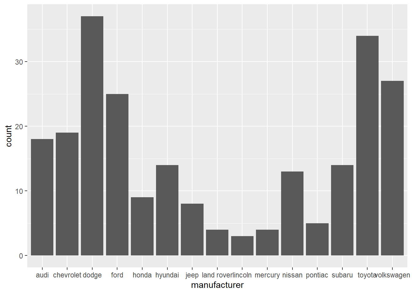

ggplot(data = mpg) +
  geom_smooth(mapping = aes(x = displ, y = hwy, size = drv))

ggplot(data = mpg, mapping = aes(x = cty, y = hwy)) +
  geom_point(mapping = aes(color = drv)) +
  geom_smooth(se = FALSE) +
  labs(title = "The Relationship Between Highway and City Fuel Efficiency",
       x = "City Fuel Efficiency (miles per gallon)",
       y = "Highway Fuel Efficiency (miles per gallon)",
       color = "Drive Train Type")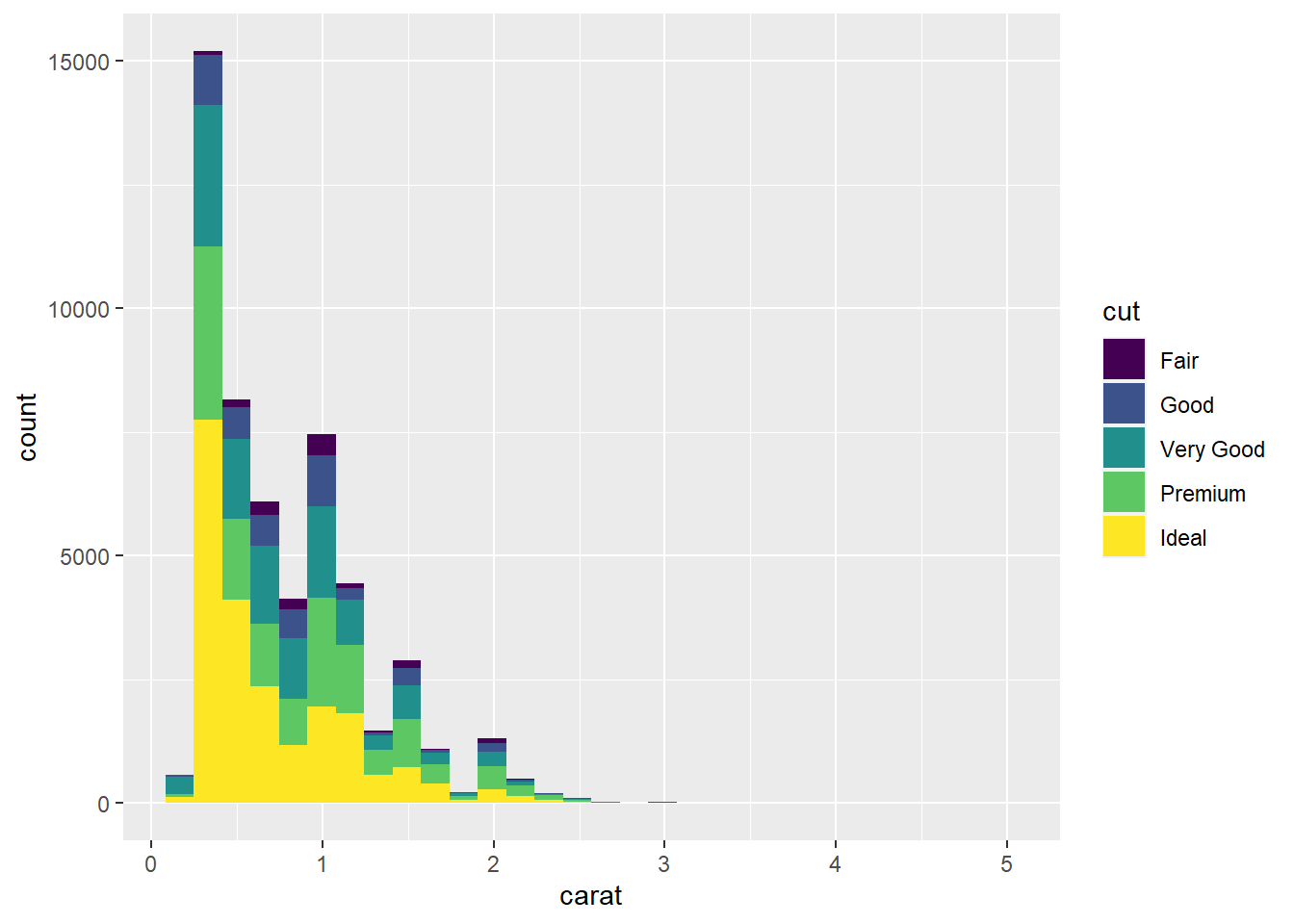

The visualization below shows that the color aesthetic should probably not be used with a categorical variable with several values since it leads to a very cluttered plot.

ggplot(data = mpg) +
  geom_smooth(mapping = aes(x = displ, y = hwy, color = class))

Section 1.6.1

Since carat and price are both continuous, a scatter plot is appropriate. Notice below that price is the y-axis variable, and carat is the x-axis variable. This is because carat is an independent variable (meaning that it’s not affected by the other variables) and price is a dependent variable (meaning that it is affected by the other variables).

ggplot(data = diamonds) +
  geom_point(mapping = aes(x = carat, y = price))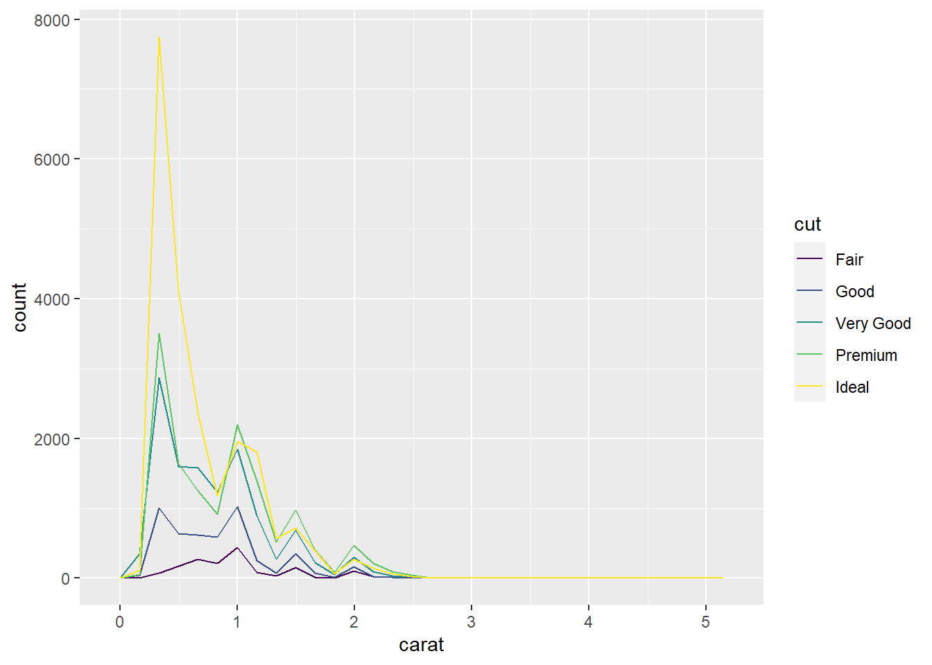

Since clarity is categorical, a better way to visualize its affect on price is to use a box plot.

ggplot(data = diamonds) +
  geom_boxplot(mapping = aes(x = clarity, y = price))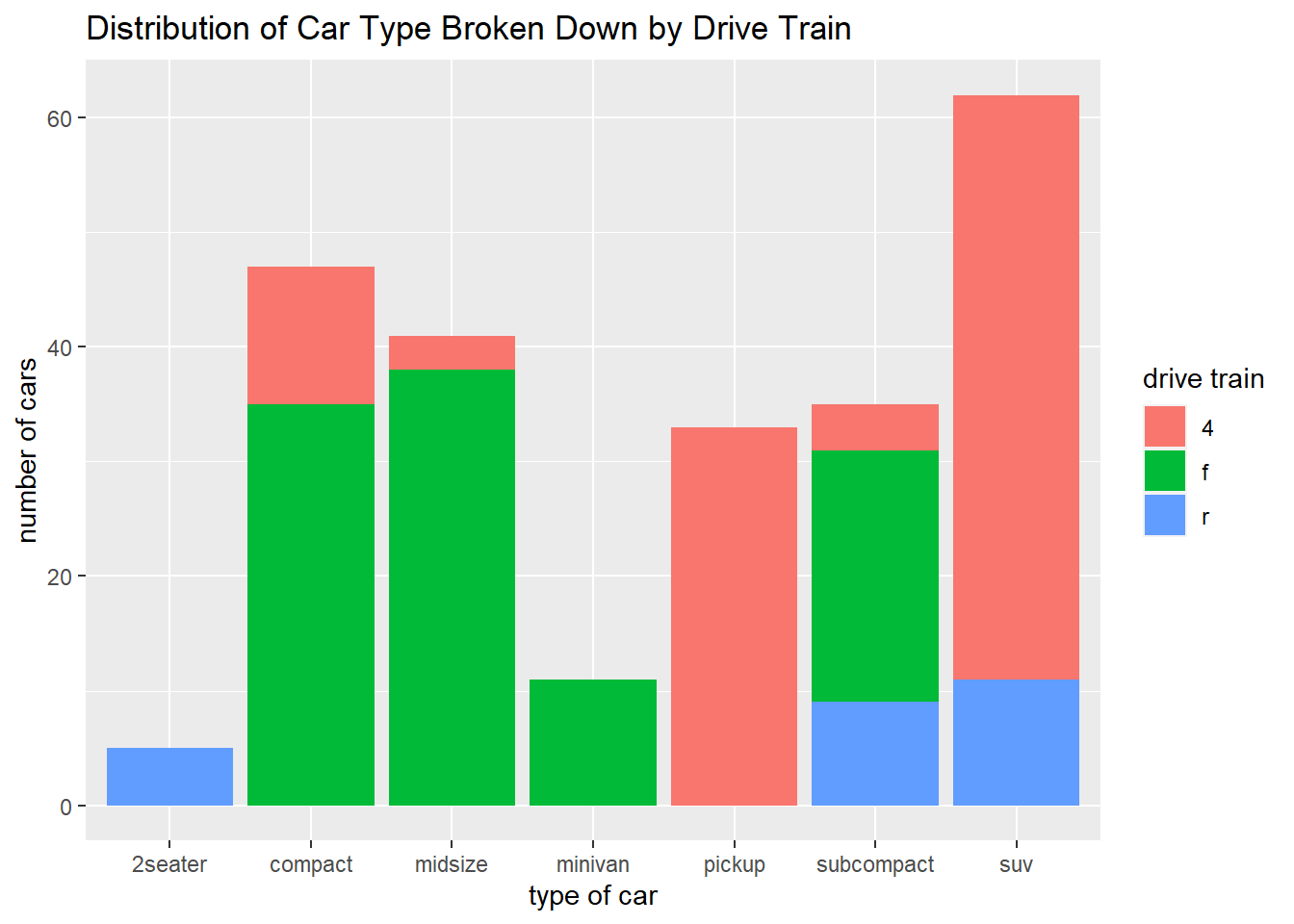

Judging by the median value of price, it looks like SI2 is the highest priced clarity value. You could also make an argument for VS2 or VS1 since they have the highest values for Q3. VS2 and VS1 clarities also seem to have the most variation in price since they have the largest interquartile ranges.
The fact that, for any given clarity value, all of the outliers lie above the main cluster indicates that the data set contains several diamonds with extremely high prices that are much larger than the median prices. This is often the case with valuable commodities - there are always several items whose values are extremely high compared to the median. (Think houses, baseball cards, cars, antiques, etc.)
The fill aesthetic seems to best among the three at visually distinguishing the values of cut.

ggplot(data = diamonds) +
  geom_boxplot(mapping = aes(x = color, y = price, color = cut))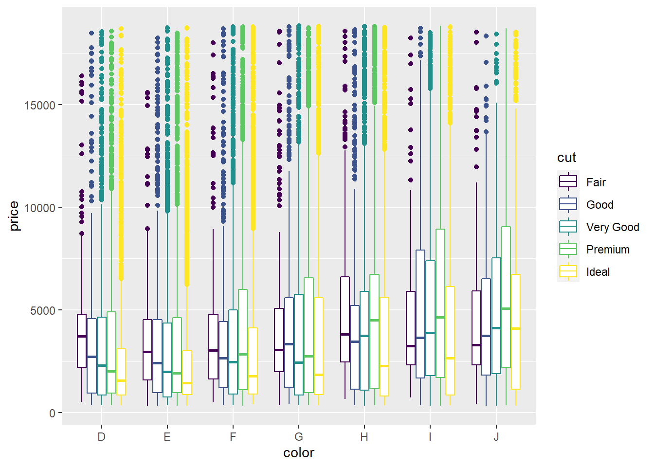

ggplot(data = diamonds) +
  geom_boxplot(mapping = aes(x = color, y = price, fill = cut))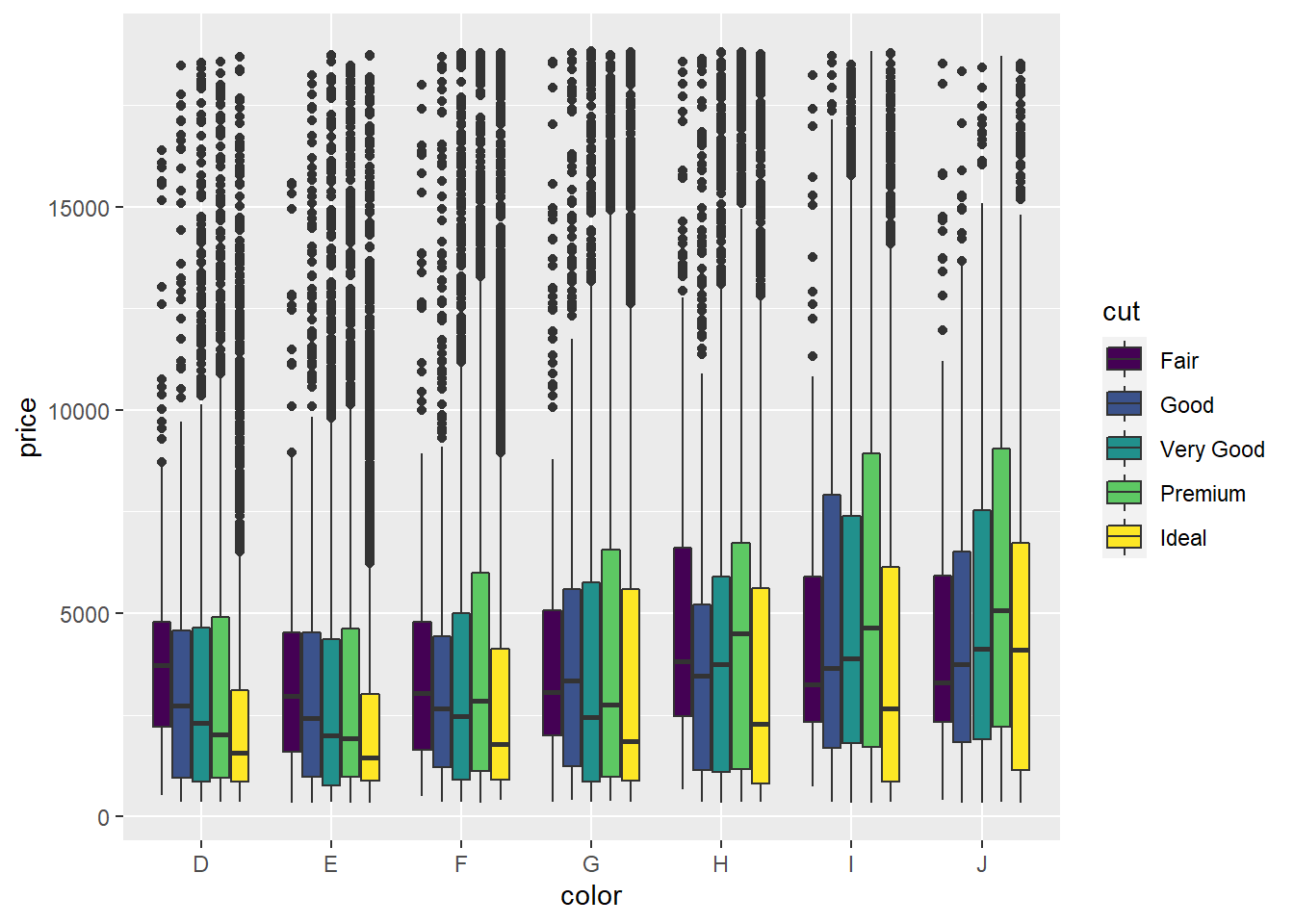

ggplot(data = diamonds) +
  geom_boxplot(mapping = aes(x = color, y = price, linetype = cut))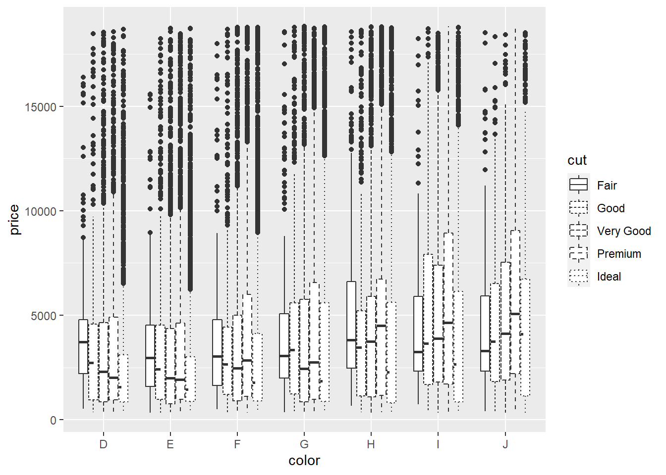

ggplot(data = diamonds) +
  geom_boxplot(mapping = aes(x = reorder(clarity, price), y = price)) +
  coord_flip()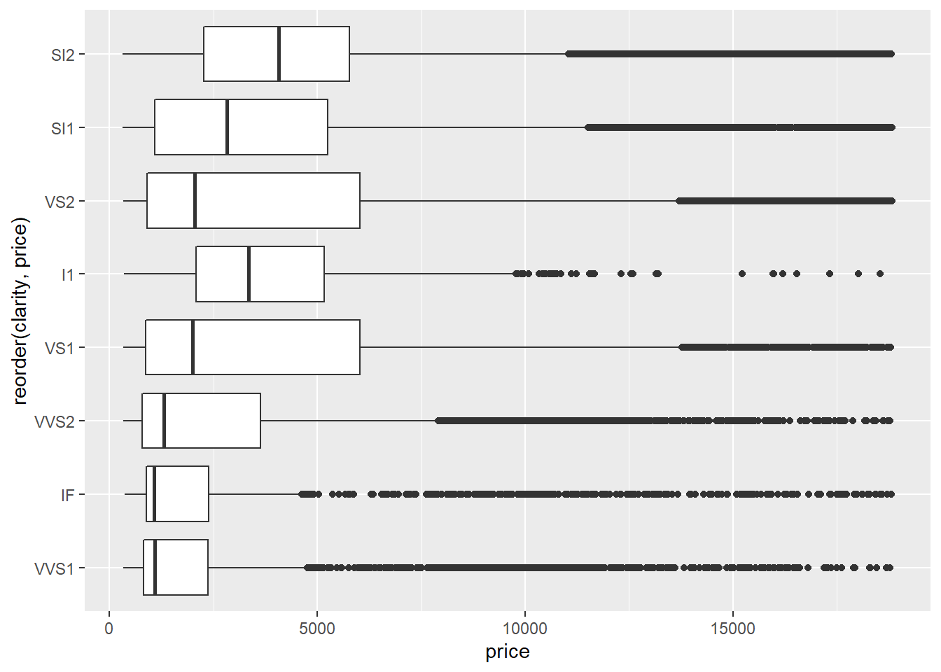

Section 1.7.1

Since clarity is categorical, we should use a bar graph.

ggplot(data = diamonds) +
  geom_bar(mapping = aes(x = clarity))

ggplot(data = diamonds) +
  geom_bar(mapping = aes(x = clarity, y = stat(prop), group = 1))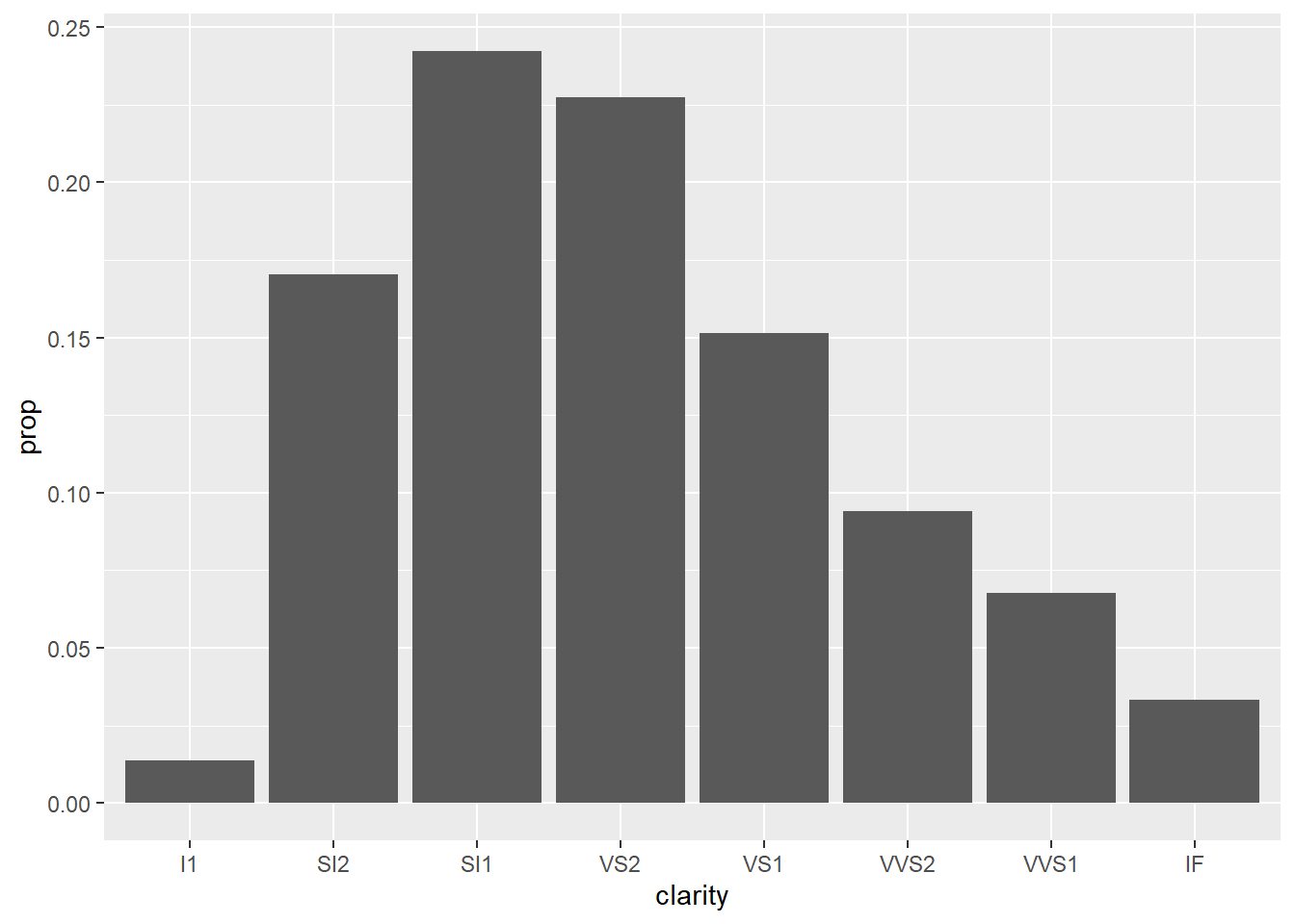

Since carat is continuous, we should now use a histogram.

ggplot(data = diamonds) +
  geom_histogram(mapping = aes(x = carat))

The first histogram below has bins that are way too narrow. The histogram is too granular to visualize the true distribution. The second one has bins which are way too wide, producing a histogram that is too coarse.

ggplot(data = diamonds) +
  geom_histogram(mapping = aes(x = carat), binwidth = 0.01)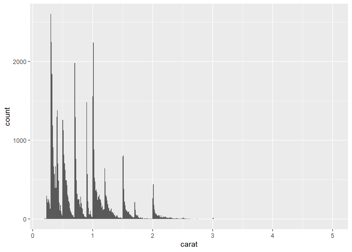

ggplot(data = diamonds) +
  geom_histogram(mapping = aes(x = carat), binwidth = 2)

The following bar graph looks so spiky because it’s producing a bar for every single value of price in the data set, of which there are hundreds, at least. Since price is continuous, a histogram would have been the way to visualize its distribution.

ggplot(data = diamonds) +
  geom_bar(mapping = aes(x = price))

Mapping cut to fill produces a much better result than mapping to color.

ggplot(data = diamonds) +
  geom_bar(mapping = aes(x = clarity, color = cut))

ggplot(data = diamonds) +
  geom_bar(mapping = aes(x = clarity, fill = cut))

Since using the optional position = "dodge" argument produces a bar for each cut value within a given clarity value, it’s easier to see how cut values are distributed within each clarity value since it allows you to compare relative counts more easily.

ggplot(data = diamonds) +
  geom_bar(mapping = aes(x = clarity, fill = cut), position = "dodge")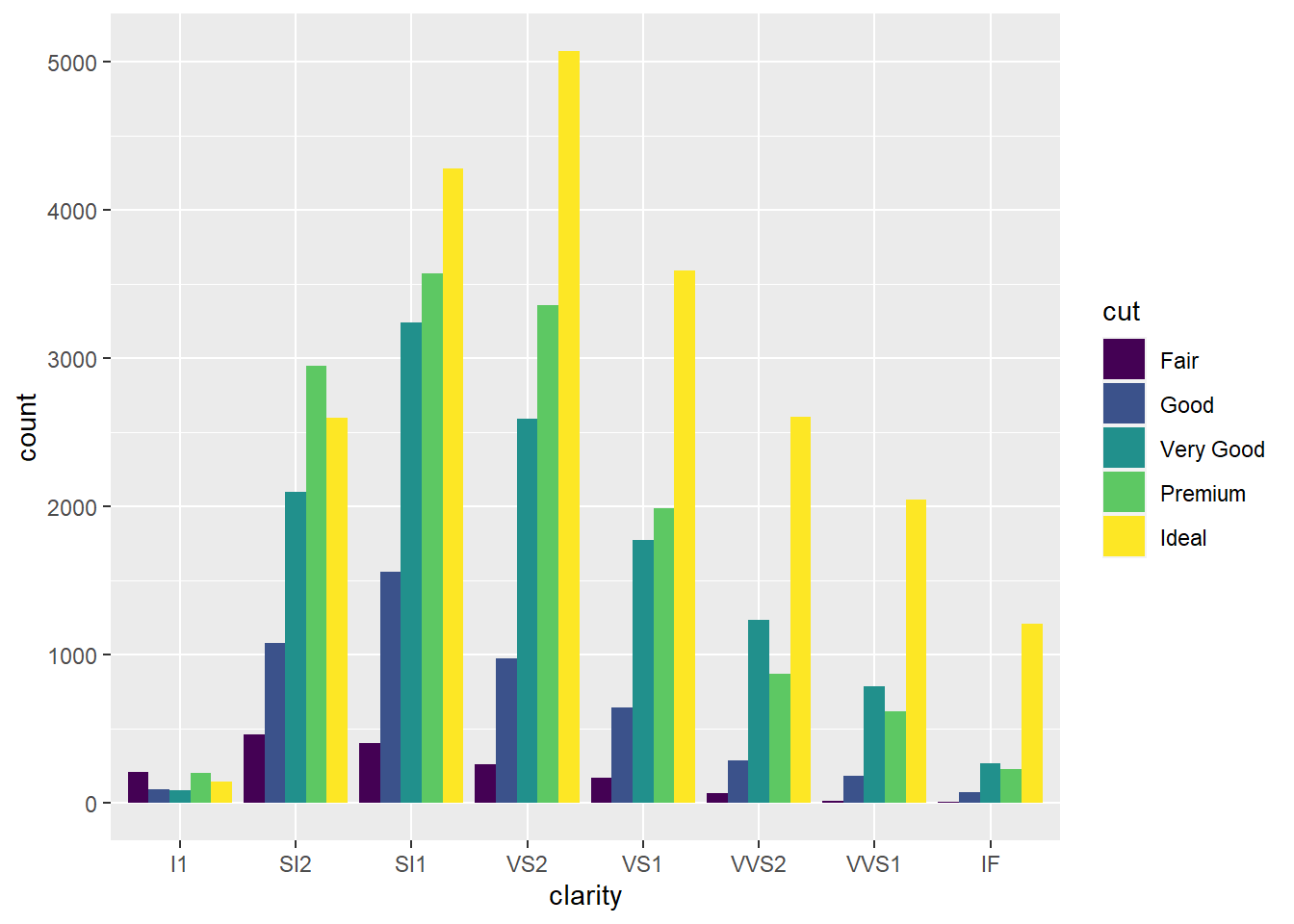

Mapping cut to two different aesthetics is redundant, but doing so makes it easier to distinguish the bars for the various cut values. (See Exercise 7 from Section 1.2.1.)

ggplot(data = diamonds) +
  geom_bar(mapping = aes(x = cut, fill = cut))

You get a pie chart, where the radius of each piece of pie corresponds to the count for that cut value.

ggplot(data = diamonds) +
  geom_bar(mapping = aes(x = cut, fill = cut)) +
  coord_polar()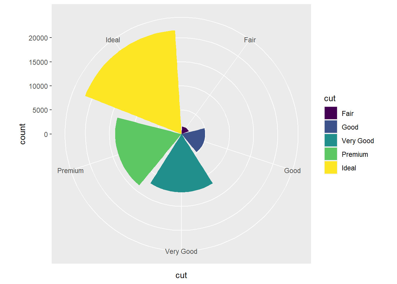

In the first bar graph below, the names of the manufacturer values are crowded together on the x-axis, making them hard to read. The second bar graph fixes this problems by adding a coord_flip() layer.

ggplot(data = mpg) +
  geom_bar(mapping = aes(x = manufacturer))

ggplot(data = mpg) +
  geom_bar(mapping = aes(x = manufacturer)) +
  coord_flip()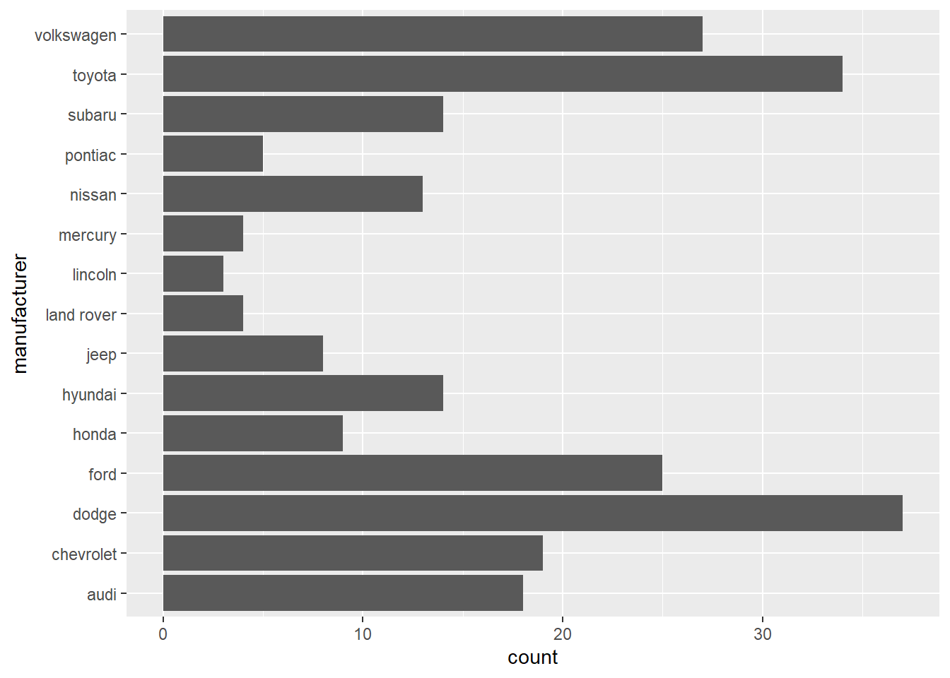

ggplot(data = diamonds) +
  geom_histogram(mapping = aes(x = carat, fill = cut))

A frequency polynomial contains the same information as a histogram but displays it in a more minimal way.

ggplot(data = diamonds) +
  geom_freqpoly(mapping = aes(x = price))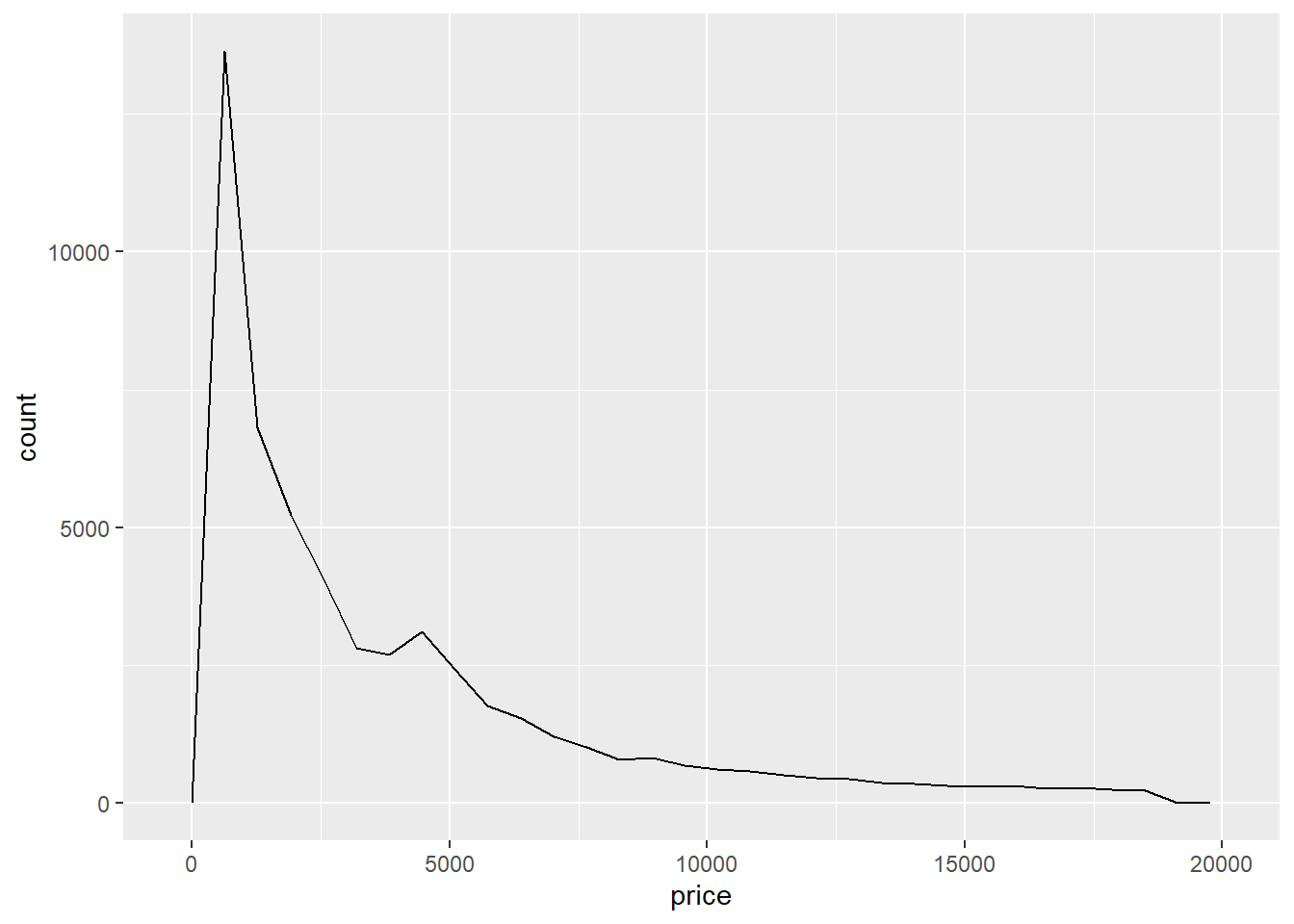

First, you may have noticed that mapping cut to fill, as was done in Exercise 11, is not as helpful in geom_freqpoly. Mapping to color produces a nice plot. It seems a little better than the histogram in Exercise 11 since it avoids the stacking of the colored segments of the bars.

ggplot(data = diamonds) +
  geom_freqpoly(mapping = aes(x = carat, color = cut))

ggplot(data = mpg) +
  geom_bar(mapping = aes(x = class, fill = drv)) +
  labs(x = "type of car",
       y = "number of cars",
       fill = "drive train",
       title = "Distribution of Car Type Broken Down by Drive Train")

Section 2.1.1

There are 336,776 observations (rows) and 19 variables (columns).

filter(flights, month == 2)

filter(flights, carrier == "UA" | carrier == "AA")

filter(flights, month >= 6 & month <= 8)

filter(flights, arr_delay > 120 & dep_delay <= 0)

filter(flights, dep_delay > 60 & dep_delay - arr_delay > 30)

filter(flights, dep_time < 600)

A canceled flight would have an NA for its departure time, so we can just count the number of NAs in this column as shown below:

sum(is.na(flights$dep_time))

## [1] 8255

We would have to find the number of flights with a 0 or negative arr_delay value and then divide that number by the total number of arriving flights Delta flew. The following shows a way to do this. (Recall that when you compute the mean of a column of TRUE/FALSE values, you’re computing the percentage of TRUEs in the column.)

# First create a data set containing the Delta flights that arrived at their destinations:
Delta_arr <- filter(flights, carrier == "DL" & !is.na(arr_delay))

# Now find the percentage of rows of this filtered data set with `arr_delay <= 0`:
mean(Delta_arr$arr_delay <= 0)

## [1] 0.6556087

So Delta’s on-time arrival rate in 2013 was about 66%. For the winter on-time arrival rate, we can repeat this calculation after filtering Delta_arr down to just the winter flights.

winter_Delta_arr <- filter(Delta_arr, month == 12 | month <= 2)

mean(winter_Delta_arr$arr_delay <= 0)

## [1] 0.6546032

The on-time arrival rate is about 65%.

Section 2.2.1

Let’s sort the msleep data set by conservation and then View it:

View(arrange(msleep, conservation))

Scrolling through the sorted data set, we see the rows with NA in the conservation column appear at the end. To move them to the top, we can do the following, remembering that is.na(conservation) will return a 1 for the rows with an NA in the conservation column and a 0 otherwise.

arrange(msleep, desc(is.na(conservation)))

The longest delay was 1301 minutes.

arrange(flights, desc(dep_delay))

## # A tibble: 336,776 x 19
##     year month   day dep_time sched_d~1 dep_d~2 arr_t~3 sched~4 arr_d~5 carrier flight tailnum origin dest 
##    <int> <int> <int>    <int>     <int>   <dbl>   <int>   <int>   <dbl> <chr>    <int> <chr>   <chr>  <chr>
##  1  2013     1     9      641       900    1301    1242    1530    1272 HA          51 N384HA  JFK    HNL  
##  2  2013     6    15     1432      1935    1137    1607    2120    1127 MQ        3535 N504MQ  JFK    CMH  
##  3  2013     1    10     1121      1635    1126    1239    1810    1109 MQ        3695 N517MQ  EWR    ORD  
##  4  2013     9    20     1139      1845    1014    1457    2210    1007 AA         177 N338AA  JFK    SFO  
##  5  2013     7    22      845      1600    1005    1044    1815     989 MQ        3075 N665MQ  JFK    CVG  
##  6  2013     4    10     1100      1900     960    1342    2211     931 DL        2391 N959DL  JFK    TPA  
##  7  2013     3    17     2321       810     911     135    1020     915 DL        2119 N927DA  LGA    MSP  
##  8  2013     6    27      959      1900     899    1236    2226     850 DL        2007 N3762Y  JFK    PDX  
##  9  2013     7    22     2257       759     898     121    1026     895 DL        2047 N6716C  LGA    ATL  
## 10  2013    12     5      756      1700     896    1058    2020     878 AA         172 N5DMAA  EWR    MIA  
## # ... with 336,766 more rows, 5 more variables: air_time <dbl>, distance <dbl>, hour <dbl>, minute <dbl>,
## #   time_hour <dttm>, and abbreviated variable names 1: sched_dep_time, 2: dep_delay, 3: arr_time,
## #   4: sched_arr_time, 5: arr_delay
## # i Use `print(n = ...)` to see more rows, and `colnames()` to see all variable names

It looks like several flights departed at 12:01am.

arrange(flights, dep_time)

## # A tibble: 336,776 x 19
##     year month   day dep_time sched_d~1 dep_d~2 arr_t~3 sched~4 arr_d~5 carrier flight tailnum origin dest 
##    <int> <int> <int>    <int>     <int>   <dbl>   <int>   <int>   <dbl> <chr>    <int> <chr>   <chr>  <chr>
##  1  2013     1    13        1      2249      72     108    2357      71 B6          22 N206JB  JFK    SYR  
##  2  2013     1    31        1      2100     181     124    2225     179 WN         530 N550WN  LGA    MDW  
##  3  2013    11    13        1      2359       2     442     440       2 B6        1503 N627JB  JFK    SJU  
##  4  2013    12    16        1      2359       2     447     437      10 B6         839 N607JB  JFK    BQN  
##  5  2013    12    20        1      2359       2     430     440     -10 B6        1503 N608JB  JFK    SJU  
##  6  2013    12    26        1      2359       2     437     440      -3 B6        1503 N527JB  JFK    SJU  
##  7  2013    12    30        1      2359       2     441     437       4 B6         839 N508JB  JFK    BQN  
##  8  2013     2    11        1      2100     181     111    2225     166 WN         530 N231WN  LGA    MDW  
##  9  2013     2    24        1      2245      76     121    2354      87 B6         608 N216JB  JFK    PWM  
## 10  2013     3     8        1      2355       6     431     440      -9 B6         739 N586JB  JFK    PSE  
## # ... with 336,766 more rows, 5 more variables: air_time <dbl>, distance <dbl>, hour <dbl>, minute <dbl>,
## #   time_hour <dttm>, and abbreviated variable names 1: sched_dep_time, 2: dep_delay, 3: arr_time,
## #   4: sched_arr_time, 5: arr_delay
## # i Use `print(n = ...)` to see more rows, and `colnames()` to see all variable names

The fastest average speed was Delta flight 1499 from LGA to ATL on May 25.

arrange(flights, desc(distance/air_time))

The slowest average speed was US Airways flight 1860 from LGA to PHL on January 28.

arrange(flights, distance/air_time)

The Hawaiian Airlines flights from JFK to HNL flew the farthest distance of 4983 miles.

arrange(flights, desc(distance))

The shortest flight in the data set was US Airways flight 1632 from EWR to LGA on July 27. (It was canceled.)

arrange(flights, distance)

Section 2.3.1

Checking the dest column of the transformed data set created below, we see that the most distant American Airlines destination is SFO.

flights %>%
  filter(carrier == "AA") %>%
  arrange(desc(distance))

We can refine the filter from the previous exercise to include only flights with LGA as the origin airport. The most distant destination is DFW.

flights %>%
  filter(carrier == "AA" & origin == "LGA") %>%
  arrange(desc(distance))

The most delayed winter flight was Hawaiian Airlines flight 51 from JFK to HNL on January 9.

flights %>%
  filter(month == 12 | month <= 2) %>%
  arrange(desc(dep_delay))

The most delayed summer flight was Envoy Air flight 3535 from JFK to CMH on June 15.

flights %>%
  filter(month >= 6 & month <= 8) %>%
  arrange(desc(dep_delay))

Section 2.5.1

The fastest flight was Delta flight 1499 from LGA to ATL on May 25. It’s average air speed was about 703 mph.

flights %>%
  filter(!is.na(dep_time)) %>%  # <---- Filters out canceled flights
  mutate(air_speed = distance/air_time * 60) %>%
  arrange(desc(air_speed)) %>%
  select(month, day, carrier, flight, origin, dest, air_speed)

The slowest flight was US Airways flight 1860 from LGA to PHL on January 28. It’s average air speed was about 77 mph.

flights %>%
  filter(!is.na(dep_time)) %>%  # <---- Filters out canceled flights
  mutate(air_speed = distance/air_time * 60) %>%
  arrange(air_speed) %>%
  select(month, day, carrier, flight, origin, dest, air_speed)

The difference column below shows the values of the the newly created flight_minutes variable minus the air_time variable already in flights. A little digging on the internet could tell us that air_time only includes the times during which the plane is actually in the air and does not include taxiing on the runway, etc. dep_time and arr_time are the times when the plane departs from and arrives at the gate, so flight_minutes includes time spent on the runway. This would mean flight_minutes should be consistently larger than air_time, producing all positive values in the difference column.

However, this is not what we observe. If we look carefully at the flights with a negative difference value, we might notice that the destination airport is not in the Eastern Time Zone. The arr_time values in the Central Time Zone are thus 60 minutes behind Eastern, Mountain Time Zone arr_times are 120 minutes behind, and Pacific Time Zones are 180 minutes behind. This explains the negative difference values and also why you would see, for example, a flight from Newark to San Francisco with a flight_minutes value of only 205.

flights %>%
  mutate(dep_mins_midnight = (dep_time %/% 100)*60 + (dep_time %% 100),
         arr_mins_midnight = (arr_time %/% 100)*60 + (arr_time %% 100),
         flight_minutes = arr_mins_midnight - dep_mins_midnight,
         difference = flight_minutes - air_time) %>%
  select(month, day, origin, dest, air_time, flight_minutes, difference)

## # A tibble: 336,776 x 7
##    month   day origin dest  air_time flight_minutes difference
##    <int> <int> <chr>  <chr>    <dbl>          <dbl>      <dbl>
##  1     1     1 EWR    IAH        227            193        -34
##  2     1     1 LGA    IAH        227            197        -30
##  3     1     1 JFK    MIA        160            221         61
##  4     1     1 JFK    BQN        183            260         77
##  5     1     1 LGA    ATL        116            138         22
##  6     1     1 EWR    ORD        150            106        -44
##  7     1     1 EWR    FLL        158            198         40
##  8     1     1 LGA    IAD         53             72         19
##  9     1     1 JFK    MCO        140            161         21
## 10     1     1 LGA    ORD        138            115        -23
## # ... with 336,766 more rows
## # i Use `print(n = ...)` to see more rows

The first day of the year with a canceled flight was January 1.

flights %>%
  mutate(status = ifelse(is.na(dep_time), "canceled", "not canceled")) %>%
  arrange(status)

## # A tibble: 336,776 x 20
##     year month   day dep_time sched_d~1 dep_d~2 arr_t~3 sched~4 arr_d~5 carrier flight tailnum origin dest 
##    <int> <int> <int>    <int>     <int>   <dbl>   <int>   <int>   <dbl> <chr>    <int> <chr>   <chr>  <chr>
##  1  2013     1     1       NA      1630      NA      NA    1815      NA EV        4308 N18120  EWR    RDU  
##  2  2013     1     1       NA      1935      NA      NA    2240      NA AA         791 N3EHAA  LGA    DFW  
##  3  2013     1     1       NA      1500      NA      NA    1825      NA AA        1925 N3EVAA  LGA    MIA  
##  4  2013     1     1       NA       600      NA      NA     901      NA B6         125 N618JB  JFK    FLL  
##  5  2013     1     2       NA      1540      NA      NA    1747      NA EV        4352 N10575  EWR    CVG  
##  6  2013     1     2       NA      1620      NA      NA    1746      NA EV        4406 N13949  EWR    PIT  
##  7  2013     1     2       NA      1355      NA      NA    1459      NA EV        4434 N10575  EWR    MHT  
##  8  2013     1     2       NA      1420      NA      NA    1644      NA EV        4935 N759EV  EWR    ATL  
##  9  2013     1     2       NA      1321      NA      NA    1536      NA EV        3849 N13550  EWR    IND  
## 10  2013     1     2       NA      1545      NA      NA    1910      NA AA         133 <NA>    JFK    LAX  
## # ... with 336,766 more rows, 6 more variables: air_time <dbl>, distance <dbl>, hour <dbl>, minute <dbl>,
## #   time_hour <dttm>, status <chr>, and abbreviated variable names 1: sched_dep_time, 2: dep_delay,
## #   3: arr_time, 4: sched_arr_time, 5: arr_delay
## # i Use `print(n = ...)` to see more rows, and `colnames()` to see all variable names

There were 9430 flights for which arr_status is NA. The reason that NA was assigned to arr_status for these flights is that the arr_delay value for these flights is NA, so the condition in the ifelse would be checking whether NA <= 0. The result of this condition can be neither TRUE nor FALSE, it will instead just be NA.

flights_w_arr_status <- flights %>%
  mutate(arr_status = ifelse(arr_delay <= 0, 
                             "on time", 
                             "late"))

sum(is.na(flights_w_arr_status$arr_status))

## [1] 9430

We will rearrange the conditions so that the first one checked is arr_delay <= 0 and the second one is is.na(arr_delay). We can then find a row with an NA in the arr_delay column by sorting by is.na(arr_delay) in descending order.

The results below show that arr_status was not correctly assigned a “canceled” value for these flights. This is because the first condition in the nested ifelse is arr_delay <= 0. As we saw in the previous exercise, when the arr_delay value is NA, this first condition is neither TRUE nor FALSE, so neither of the conditional statements will be executed. Instead, a value of NA will be assigned to arr_status.

flights_w_arr_status2 <- flights %>%
  mutate(arr_status = ifelse(arr_delay <= 0, 
                             "on time",
                             ifelse(is.na(arr_delay),
                                    "canceled",
                                    "late"))) %>%
  arrange(desc(is.na(arr_delay))) %>%
  select(arr_delay, arr_status)

flights_w_arr_status2

## # A tibble: 336,776 x 2
##    arr_delay arr_status
##        <dbl> <chr>     
##  1        NA <NA>      
##  2        NA <NA>      
##  3        NA <NA>      
##  4        NA <NA>      
##  5        NA <NA>      
##  6        NA <NA>      
##  7        NA <NA>      
##  8        NA <NA>      
##  9        NA <NA>      
## 10        NA <NA>      
## # ... with 336,766 more rows
## # i Use `print(n = ...)` to see more rows

We’ll interchange the first two conditions as we did in the previous exercise and then again sort by is.na(arr_status) in descending order to find the flights for which arr_delay is NA. We can see that arr_status is correctly assigned a canceled value. This shows that the order in which the conditions are listed does not matter in a case_when statement. The previous exercise shows that the order does matter in a nested ifelse, which means that case_when statements are more robust ways to handle conditional statements.

flights_w_arr_status3 <- flights %>%
  mutate(arr_status = case_when(arr_delay <= 0 ~ "on time",
                                is.na(arr_delay) ~ "canceled",
                                arr_delay >0 ~ "delayed")) %>%
  arrange(desc(is.na(arr_delay))) %>%
  select(arr_delay, arr_status)

flights_w_arr_status3

## # A tibble: 336,776 x 2
##    arr_delay arr_status
##        <dbl> <chr>     
##  1        NA canceled  
##  2        NA canceled  
##  3        NA canceled  
##  4        NA canceled  
##  5        NA canceled  
##  6        NA canceled  
##  7        NA canceled  
##  8        NA canceled  
##  9        NA canceled  
## 10        NA canceled  
## # ... with 336,766 more rows
## # i Use `print(n = ...)` to see more rows

flights %>%
  mutate(season = case_when(month >= 3 & month <= 5 ~ "spring",
                            month >= 6 & month <= 8 ~ "summer",
                            month >= 9 & month <= 11 ~ "fall",
                            TRUE ~ "winter"))

It might help to recall the distribution of price in diamonds by looking at its histogram shown below.

ggplot(data = diamonds) +
  geom_histogram(mapping = aes(x = price))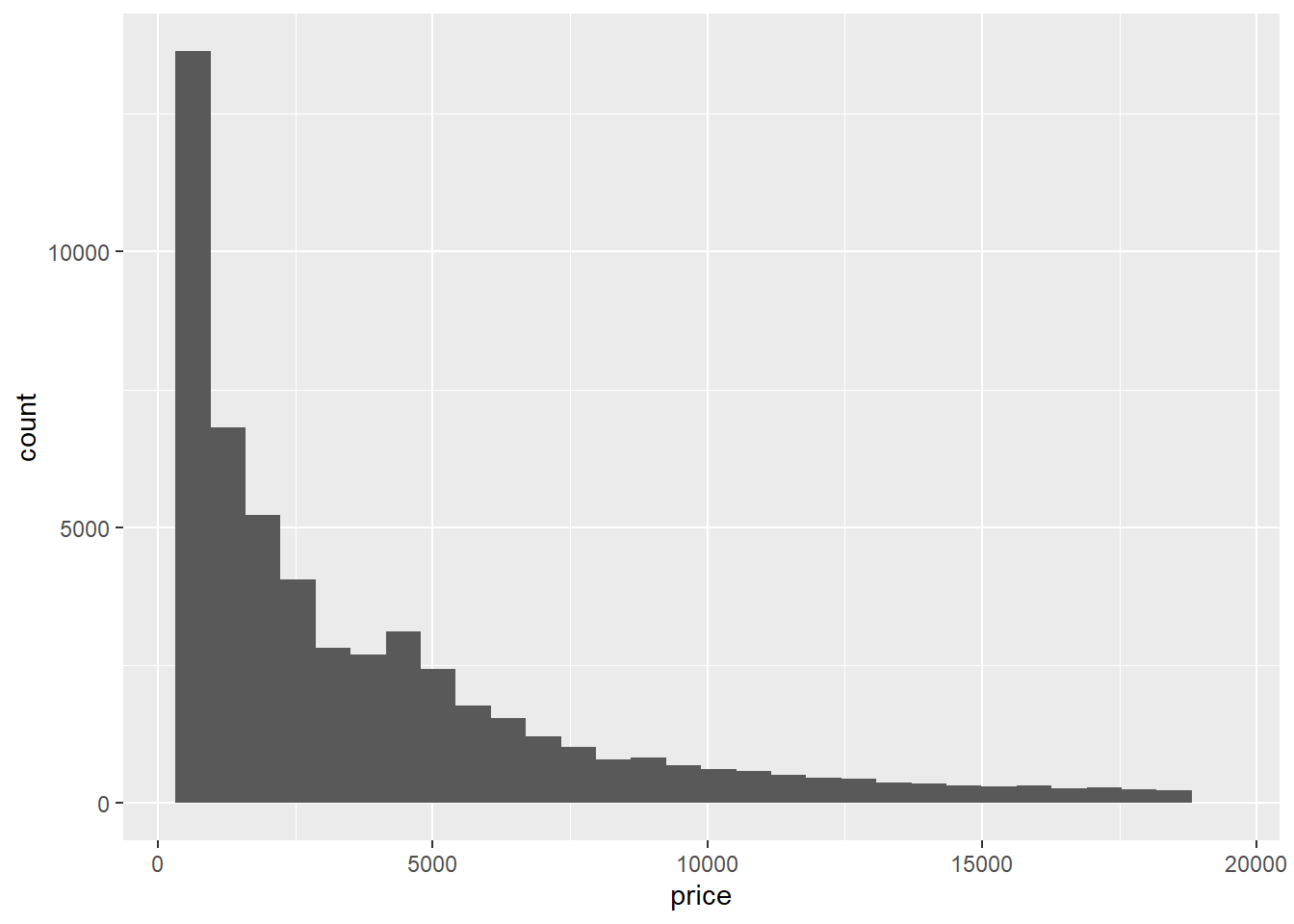

The histogram might suggest the following cutoffs: expensive for price < 5000, very expensive for 5000 <= price < 10000, insanely expensive for 10000 <= price < 15000 and priceless for price >= 15000. We can assign these labels with the following case_when:

diamonds2 <- diamonds %>%
  mutate(category = case_when(price < 5000 ~ "expensive",
                           price >= 5000 & price < 10000 ~ "very expensive",
                           price >= 10000 & price < 15000 ~ "insanely expensive",
                           TRUE ~ "priceless"))

Finally, we can visualize the distribution with a bar graph:

ggplot(data = diamonds2) +
  geom_bar(mapping = aes(x = category))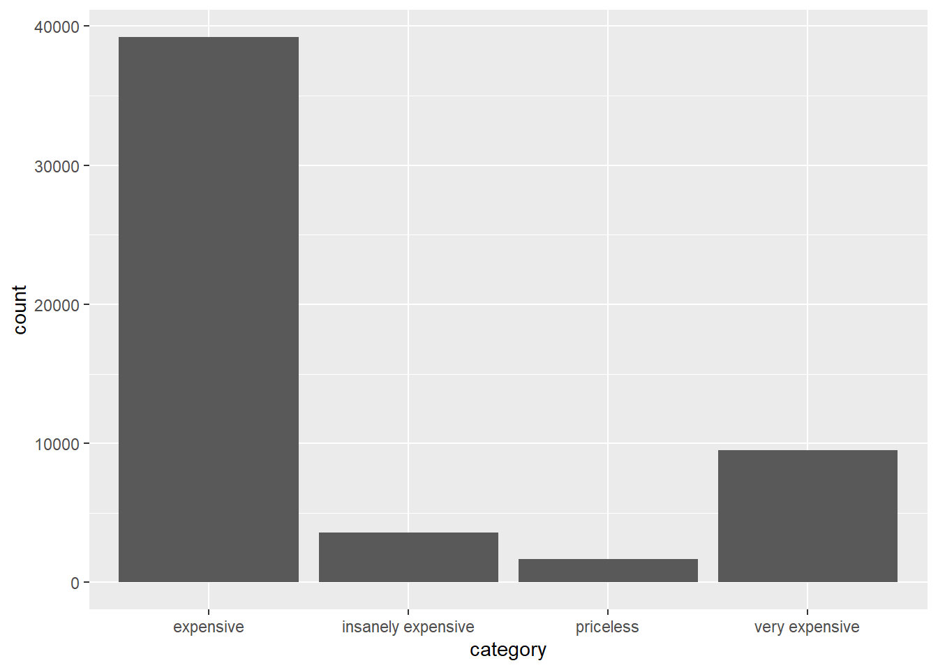

Batting has 110,495 observations and 22 variables.
Our results are surprising because there are several players with perfect batting averages. This is explained by the fact that these players had very few at bats.

Batting %>%
  mutate(batting_average = H/AB) %>%
  arrange(desc(batting_average))

The highest single season batting average of 0.440 belonged to Hugh Duffy in 1894.

Batting %>%
  filter(AB >= 350) %>%
  mutate(batting_average = H/AB) %>%
  arrange(desc(batting_average))

The highest batting average of the modern era belonged to Tony Gwynn, who hit 0.394 in 1994.

Batting %>%
  filter(yearID >= 1947,
         AB >= 350) %>%
  mutate(batting_average = H/AB) %>%
  arrange(desc(batting_average))

The last player to hit 0.400 was Ted Williams in 1941.

Batting %>%
  filter(AB >= 350) %>%
  mutate(batting_average = H/AB) %>%
  filter(batting_average >= 0.4) %>%
  arrange(desc(yearID))

Section 2.6.1

Be sure to remove the NA values when computing the mean.

flights %>%
  group_by(month, day) %>%
  summarize(avg_dep_delay = mean(dep_delay, na.rm = TRUE))

The carrier with the best on-time rate was AS (Alaska Airlines) at about 73%. However, American Airlines and Delta Airlines should be recognized as well since they maintained comparably high on-time rates while flying tens of thousands more flights than Alaska Airlines.

The carrier with the worst on-time rate was FL (Airtran Airways) at about 40%. It should also be mentioned that Express Jet (EV) flew over 50,000 flights while compiling an on-time rate of just 52%.

arr_rate <- flights %>%
  group_by(carrier) %>%
  summarize(on_time_rate = mean(arr_delay <= 0, na.rm = TRUE),
            count = n())

arrange(arr_rate, desc(on_time_rate))

## # A tibble: 16 x 3
##    carrier on_time_rate count
##    <chr>          <dbl> <int>
##  1 AS             0.733   714
##  2 HA             0.716   342
##  3 AA             0.665 32729
##  4 VX             0.659  5162
##  5 DL             0.656 48110
##  6 OO             0.655    32
##  7 US             0.629 20536
##  8 9E             0.616 18460
##  9 UA             0.615 58665
## 10 B6             0.563 54635
## 11 WN             0.560 12275
## 12 MQ             0.533 26397
## 13 YV             0.526   601
## 14 EV             0.521 54173
## 15 F9             0.424   685
## 16 FL             0.403  3260

arrange(arr_rate, on_time_rate)

## # A tibble: 16 x 3
##    carrier on_time_rate count
##    <chr>          <dbl> <int>
##  1 FL             0.403  3260
##  2 F9             0.424   685
##  3 EV             0.521 54173
##  4 YV             0.526   601
##  5 MQ             0.533 26397
##  6 WN             0.560 12275
##  7 B6             0.563 54635
##  8 UA             0.615 58665
##  9 9E             0.616 18460
## 10 US             0.629 20536
## 11 OO             0.655    32
## 12 DL             0.656 48110
## 13 VX             0.659  5162
## 14 AA             0.665 32729
## 15 HA             0.716   342
## 16 AS             0.733   714

One way we can answer this question by comparing the minimum air_time value to the average air_time value at each destination and sorting by the difference to find destinations with minimums way smaller than averages.

It looks like there was a flight to Minneapolis-St. Paul that arrived almost 1 hour faster than the average flight to that destination. (It looks like this flight left the origin gate at 3:58PM EST and arrived at the destination gate at 5:45PM CST, which would mean 107 minutes gate-to-gate. The air_time value of 93 is thus probably not an entry error. The flight had a departure delay of 45 minutes and may have been trying to make up time in the air.)

flights %>%
  filter(!is.na(air_time)) %>%
  group_by(dest) %>%
  summarize(min_air_time = min(air_time),
            avg_air_time = mean(air_time)) %>%
  arrange(desc(avg_air_time - min_air_time))

Express Jet flew to 61 different destinations.

flights %>%
  group_by(carrier) %>%
  summarize(dist_dest = n_distinct(dest)) %>%
  arrange(desc(dist_dest))

Standard deviation is the statistic most often used to measure variation in a variable. The plane with tail number N76062 had the highest standard deviation is distances flown at about 1796 miles.

flights %>%
  filter(!is.na(tailnum)) %>%
  group_by(tailnum) %>%
  summarize(variation = sd(distance, na.rm = TRUE),
            count = n()) %>%
  arrange(desc(variation))

February 8 had the most cancellations at 472. There were 7 days with no cancellations, including, luckily, Thanksgiving and the day after Thanksgiving.

cancellations <- flights %>%
  group_by(month, day) %>%
  summarize(flights_canceled = sum(is.na(dep_time)))

arrange(cancellations, desc(flights_canceled))

## # A tibble: 365 x 3
## # Groups:   month [12]
##    month   day flights_canceled
##    <int> <int>            <int>
##  1     2     8              472
##  2     2     9              393
##  3     5    23              221
##  4    12    10              204
##  5     9    12              192
##  6     3     6              180
##  7     3     8              180
##  8    12     5              158
##  9    12    14              125
## 10     6    28              123
## # ... with 355 more rows
## # i Use `print(n = ...)` to see more rows

arrange(cancellations, flights_canceled)

## # A tibble: 365 x 3
## # Groups:   month [12]
##    month   day flights_canceled
##    <int> <int>            <int>
##  1     4    21                0
##  2     5    17                0
##  3     5    26                0
##  4    10     5                0
##  5    10    20                0
##  6    11    28                0
##  7    11    29                0
##  8     1     6                1
##  9     1    19                1
## 10     2    16                1
## # ... with 355 more rows
## # i Use `print(n = ...)` to see more rows

HR_by_year <- Batting %>% 
  group_by(yearID) %>%
  summarize(max_HR = max(HR))

The huge jump around 1920 is explained by the arrival of Babe Ruth. Home runs totals remained very high in his aftermath, showing how dramatically he changed the game. You might also recognize some high spikes during the PED-fueled years of Mark McGwire, Sammy Sosa, and Barry Bonds, and some low spikes during strike- or COVID- shortened seasons.

ggplot(data = HR_by_year, mapping = aes(x = yearID, y = max_HR)) +
  geom_point() +
  geom_line()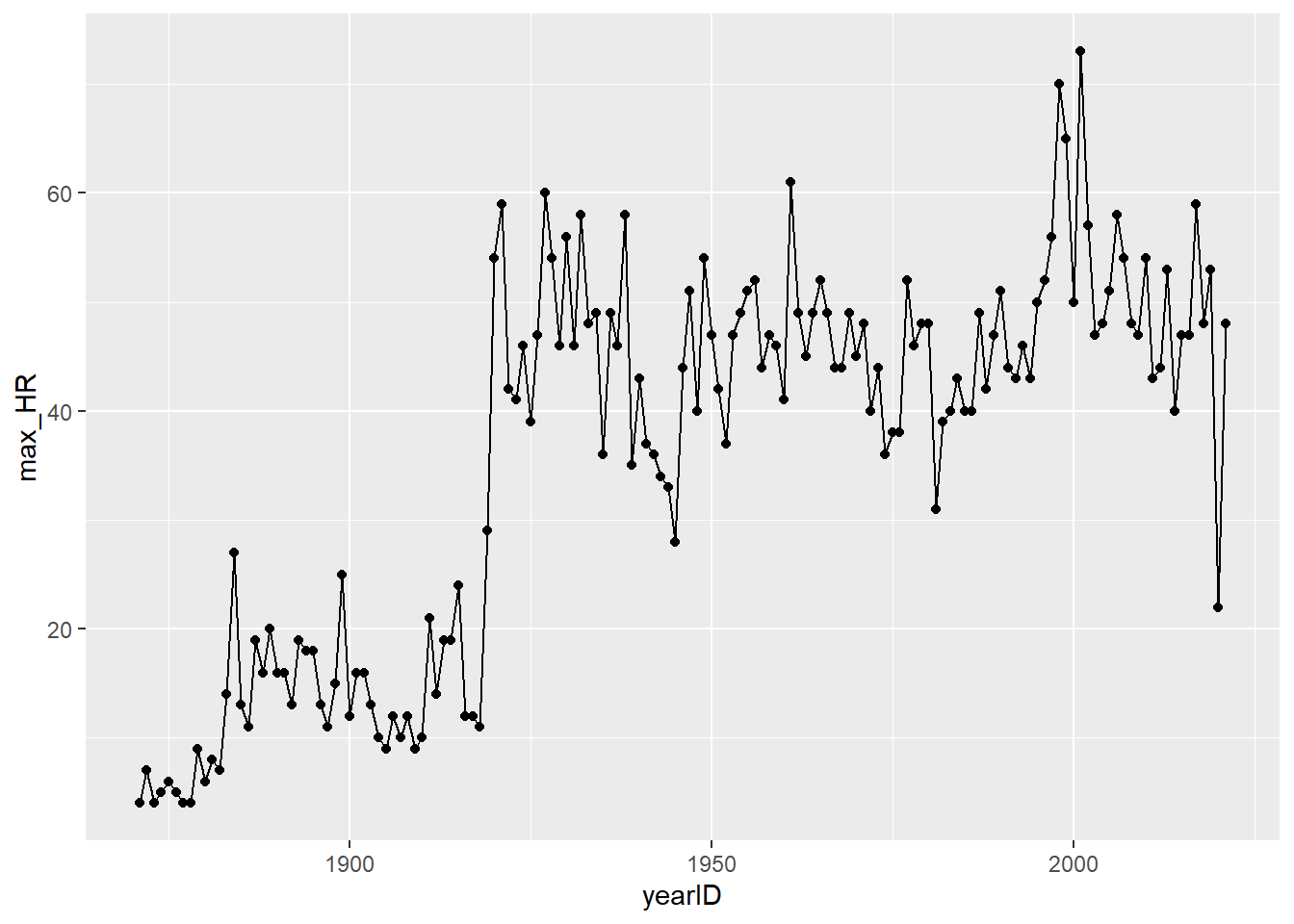

Batting %>%
  group_by(playerID) %>%
  summarize(at_bats = sum(AB, na.rm = TRUE),
            hits = sum(H, na.rm = TRUE),
            batting_avg = hits/at_bats) %>%
  filter(at_bats >= 3000) %>%
  arrange(desc(batting_avg))

## # A tibble: 1,774 x 4
##    playerID  at_bats  hits batting_avg
##    <chr>       <int> <int>       <dbl>
##  1 cobbty01    11436  4189       0.366
##  2 hornsro01    8173  2930       0.358
##  3 jacksjo01    4981  1772       0.356
##  4 odoulle01    3264  1140       0.349
##  5 delahed01    7510  2597       0.346
##  6 speaktr01   10195  3514       0.345
##  7 hamilbi01    6283  2164       0.344
##  8 willite01    7706  2654       0.344
##  9 broutda01    6726  2303       0.342
## 10 ruthba01     8398  2873       0.342
## # ... with 1,764 more rows
## # i Use `print(n = ...)` to see more rows

Section 3.1.1

The code to import the file is sample_xlsx <- read_excel("sample_xlsx.xlsx"). You are also required to load the readxl library. This is different from the previous imports in that the file is an Excel spreadsheet, and thus the read_excel function is required instead of read_csv.
A more descriptive name for this data set would be colleges. We should also uncheck the box that says, “First Row as Names” on the import screen. The code to import it with these adjustments is colleges <- read_excel("sample_2.xlsx", col_names = FALSE).
The columns name assigned were ...1, ...2, and ...3. You can specify your own column names during the import as follows:

colleges <- read_excel("sample_2.xlsx", col_names = c("college", "city", "state"))

schedule <- tribble(
  ~course, ~title, ~credits,
  "MS 121", "Calculus I", 4,
  "MS 231", "Multivariable Calculus", 3,
  "MS 282", "Applied Statistics with R", 3
)

Section 3.2.1

The variable time_hour has a type of “dttm.” This stands for “date-time” and is a combination of a date and a time.

mpg2 <- mpg %>%
  mutate(hwy = as.double(hwy),
         cty = as.double(cty))

1. Coercing an integer into a character returns a one-character string consisting of the symbol for the integer. It will no longer have a numberical value. For example, as.character(7L) returns "7".
2. The same thing happens as in part (a). For example, as.character(2.8) returns "2.8".
3. Coercing a double into an integer returns the integer part of the number. For example, as.integer(2.8) returns 2.
4. Coercing a character value containing letters into either a double or an integer returns NA. You can try this on a specific example such as as.integer("q") or as.double("q"). However, if the character is actually a number, then coercing it into an integer or double restores its numerical value. For example, as.integer("7") returns the number 7, and as.double("7.7") returns the number 7.7.
1. day is a double, but it should be an integer.
2. We’ll have to change month to a factor where the levels are the months in chronological order.

# part (a)

holidays <- read_csv("holidays.csv")

holidays <- holidays %>%
  mutate(day = as.integer(day))

# part (b)

month_levels <- c("Jan", "Feb", "Mar", "Apr", "May", "Jun", 
                  "Jul", "Aug", "Sep", "Oct", "Nov", "Dec")

holidays <- holidays %>%
  mutate(month = factor(month, levels = month_levels)) %>%
  arrange(month, day)

holidays

## # A tibble: 9 x 3
##   month   day holiday                    
##   <fct> <int> <chr>                      
## 1 Jan       1 New Year's Day             
## 2 Jan      18 Martin Luther King, Jr. Day
## 3 Feb      14 Valentine's Day            
## 4 Feb      15 President's Day            
## 5 Mar      17 St. Patrick's Day          
## 6 Jul       4 Independence Day           
## 7 Jul      14 Bastille Day               
## 8 Oct      31 Halloween                  
## 9 Dec      25 Christmas

Section 3.3.1

high_school_data_clean <- high_school_data %>%
  rename("Acad_Standing" = `Acad Standing After FA20 (Dean's List, Good Standing, Academic Warning, Academic Probation, Academic Dismissal, Readmission on Condition)`,
         "hs_qual_acad" = `High School Quality Academic`,
         "FA20_cr_hrs_att" = `FA20 Credit Hours Attempted`,
         "FA20_cr_hrs_earned" = `FA20 Credit Hours Earned`)

Section 3.4.1

The NAs in the other columns should probably not be replaced. Doing so would require too much speculation on the analyst’s part.
There is no NA count for the categorical variables.

sum(is.na(high_school_data_clean$`Bridge Program?`))

## [1] 266

sum(is.na(high_school_data_clean$Acad_Standing))

## [1] 0

sum(is.na(high_school_data_clean$Race))

## [1] 21

sum(is.na(high_school_data_clean$Ethnicity))

## [1] 7

high_school_data_clean <- high_school_data_clean %>%
  mutate(converted_ACT = 41.6*`ACT Comp` + 102.4)

high_school_data_clean <- high_school_data_clean %>%
  mutate(best_score = pmax(`SAT Comp`, converted_ACT, na.rm = TRUE))

Batting_PA <- Batting %>%
  mutate(PA = AB + BB + IBB + HBP + SH + SF)

b. There are several missing values in the `IBB`, `HBP`, `SH`, and `SF` columns. When one of these values is missing, any sum that contains it as a summand will be reported as `NA`.

c.

sum(is.na(Batting$AB))

## [1] 0

sum(is.na(Batting$BB))

## [1] 0

sum(is.na(Batting$IBB))

## [1] 36650

sum(is.na(Batting$HBP))

## [1] 2816

sum(is.na(Batting$SH))

## [1] 6068

sum(is.na(Batting$SF))

## [1] 36103

d.

Batting_PA <- Batting %>%
  mutate(IBB = replace_na(IBB, 0),
         HBP = replace_na(HBP, 0),
         SH = replace_na(SH, 0),
         SF = replace_na(SF, 0))

e.

Batting_PA <- Batting_PA %>%
  mutate(PA = AB + BB + IBB + HBP + SH + SF)
    
sum(is.na(Batting_PA$PA))

## [1] 0

f. The single season record-holder for plate appearances is Pete Rose in 1974, with a total of 784.

Batting_PA %>%
  arrange(desc(PA))

##     playerID yearID stint teamID lgID   G  AB   R   H X2B X3B HR RBI  SB CS  BB  SO IBB HBP SH SF GIDP  PA
## 1   rosepe01   1974     1    CIN   NL 163 652 110 185  45   7  3  51   2  4 106  54  14   5  1  6    9 784
## 2  rolliji01   2007     1    PHI   NL 162 716 139 212  38  20 30  94  41  6  49  85   5   7  0  6   11 783
## 3  dykstle01   1993     1    PHI   NL 161 637 143 194  44   6 19  66  37 12 129  64   9   2  0  5    8 782
## 4  suzukic01   2004     1    SEA   AL 161 704 101 262  24   5  8  60  36 11  49  63  19   4  2  3    6 781
## 5  reyesjo01   2007     1    NYN   NL 160 681 119 191  36  12 12  57  78 21  77  78  13   1  5  1    6 778
## 6   rosepe01   1975     1    CIN   NL 162 662 112 210  47   4  7  74   0  1  89  50   8  11  1  1   13 772
## 7   cashda01   1975     1    PHI   NL 162 699 111 213  40   3  4  57  13  6  56  34   5   4  0  7    8 771
## 8  vaughmo01   1996     1    BOS   AL 161 635 118 207  29   1 44 143   2  0  95 154  19  14  0  8   17 771
## 9  reyesjo01   2008     1    NYN   NL 159 688 113 204  37  19 16  68  56 15  66  82   8   1  5  3    9 771
## 10 suzukic01   2006     1    SEA   AL 161 695 110 224  20   9  9  49  45  2  49  71  16   5  1  2    2 768
## 11  rosepe01   1976     1    CIN   NL 162 665 130 215  42   6 10  63   9  5  86  54   7   6  0  2   17 766
## 12 morenom01   1979     1    PIT   NL 162 695 110 196  21  12  8  69  77 21  51 104   9   3  6  2    7 766
## 13 molitpa01   1991     1    ML4   AL 158 665 133 216  32  13 17  75  19  8  77  62  16   6  0  1   11 765
## 14 boggswa01   1985     1    BOS   AL 161 653 107 240  42   3  8  78   2  1  96  61   5   4  3  2   20 763
## 15 anderbr01   1992     1    BAL   AL 159 623 100 169  28  10 21  80  53 16  98  98  14   9 10  9    2 763
## 16 suzukic01   2005     1    SEA   AL 162 679 111 206  21  12 15  68  33  8  48  66  23   4  2  6    5 762
## 17 boggswa01   1989     1    BOS   AL 156 621 113 205  51   7  3  54   2  6 107  51  19   7  0  7   19 761
## 18 suzukic01   2008     1    SEA   AL 162 686 103 213  20   7  6  42  43  4  51  65  12   5  3  4    8 761
## 19 willsma01   1962     1    LAN   NL 165 695 130 208  13  10  6  48 104 13  51  57   1   2  7  4    7 760
## 20 rolliji01   2006     1    PHI   NL 158 689 127 191  45   9 25  83  36  4  57  80   2   5  0  7   12 760
## 21  rosepe01   1965     1    CIN   NL 162 670 117 209  35  11 11  81   8  3  69  76   2   8  8  2   10 759
## 22 sizemgr01   2006     1    CLE   AL 162 655 134 190  53  11 28  76  22  6  78 153   8  13  1  4    2 759
## 23 sizemgr01   2008     1    CLE   AL 157 634 101 170  39   5 33  90  38  5  98 130  14  11  0  2    5 759
## 24  rosepe01   1973     1    CIN   NL 160 680 115 230  36   8  5  64  10  7  65  42   6   6  1  0   14 758
## 25 biggicr01   1999     1    HOU   NL 160 639 123 188  56   0 16  73  28 14  88 107   9  11  5  6    5 758
## 26 crosefr01   1938     1    NYA   AL 157 631 113 166  35   3  9  55  27 12 106  97   0  15  5  0   NA 757
## 27 sizemgr01   2007     1    CLE   AL 162 628 118 174  34   5 24  78  33 10 101 155   9  17  0  2    3 757
## 28 dimagdo01   1948     1    BOS   AL 155 648 127 185  40   4  9  87  10  2 101  58   0   2  5  0   11 756
## 29 morenom01   1980     1    PIT   NL 162 676  87 168  20  13  2  36  96 33  57 101  11   2  3  7    9 756
## 30 erstada01   2000     1    ANA   AL 157 676 121 240  39   6 25 100  28  8  64  82   9   1  2  4    8 756
## 31 engliwo01   1930     1    CHN   NL 156 638 152 214  36  17 14  59   3 NA 100  72   0   6 11  0   NA 755
## 32 richabo01   1962     1    NYA   AL 161 692  99 209  38   5  8  59  11  9  37  24   1   1 20  4   13 755
## 33  alouma01   1969     1    PIT   NL 162 698 105 231  41   6  1  48  22  8  42  35   9   2  1  3    5 755
## 34 suzukic01   2002     1    SEA   AL 157 647 111 208  27   8  8  51  31 15  68  62  27   5  3  5    8 755
## 35 jeterde01   2005     1    NYA   AL 159 654 122 202  25   5 19  70  14  5  77 117   3  11  7  3   15 755
## 36 weeksri01   2010     1    MIL   NL 160 651 112 175  32   4 29  83  11  4  76 184   0  25  0  2    5 754
## 37  riceji01   1978     1    BOS   AL 163 677 121 213  25  15 46 139   7  5  58 126   7   5  1  5   15 753
## 38 mattido01   1986     1    NYA   AL 162 677 117 238  53   2 31 113   0  0  53  35  11   1  1 10   17 753
## 39 douthta01   1928     1    SLN   NL 154 648 111 191  35   3  3  43  11 NA  84  36   0  10 10  0   NA 752
## 40 bondsbo01   1970     1    SFN   NL 157 663 134 200  36  10 26  78  48 10  77 189   7   2  1  2    6 752
## 41 molitpa01   1982     1    ML4   AL 160 666 136 201  26   8 19  71  41  9  69  93   1   1 10  5    9 752
## 42 gonzalu01   2001     1    ARI   NL 162 609 128 198  36   7 57 142   1  1 100  83  24  14  0  5   14 752
## 43 lindofr01   2018     1    CLE   AL 158 661 129 183  42   2 38  92  25 10  70 107   7   8  3  3    5 752
##  [ reached 'max' / getOption("max.print") -- omitted 110452 rows ]

g. The career record-holder for plate appearances is also Pete Rose, with a total of 16,028.

Batting_PA %>%
  group_by(playerID) %>%
  summarize(career_PA = sum(PA)) %>%
  arrange(desc(career_PA))

## # A tibble: 20,166 x 2
##    playerID  career_PA
##    <chr>         <dbl>
##  1 rosepe01      16028
##  2 aaronha01     14233
##  3 yastrca01     14181
##  4 henderi01     13407
##  5 bondsba01     13294
##  6 cobbty01      13071
##  7 murraed02     13039
##  8 pujolal01     13005
##  9 ripkeca01     12990
## 10 musiast01     12839
## # ... with 20,156 more rows
## # i Use `print(n = ...)` to see more rows

Section 3.5.1

It looks like there are entry errors in the SAT Comp and ACT Comp columns. The minimum SAT Comp score is 100, which is below the lowest possible score on the SAT. The minimum ACT Comp score is 4.05, which is not an integer and therefore can’t be an ACT score. We can see these from the summary statistics, histograms, and a sorted lists as follows:

# Part (a): summary statistics
summary(high_school_data)

# Part (b): histograms
ggplot(data = high_school_data) +
  geom_histogram(mapping = aes(x = `SAT Comp`))

ggplot(data = high_school_data) +
  geom_histogram(mapping = aes(x = `ACT Comp`))

# Part (c): sorted lists
head(arrange(high_school_data, `SAT Comp`))

head(arrange(high_school_data, `ACT Comp`))

Since it’s not clear what numbers the 100 and 4.05 were supposed to be, it’s not appropriate to change them.
We first have to find the spot in the SAT Comp column where the 100 is. Once we know this, we can change the value to 1000 as follows:

spot_100 <- which(high_school_data$`SAT Comp` == 100)

high_school_data$`SAT Comp`[spot_100] <- 1000

t <- c("a", "b", "c", "d", "e")

t[c(1,4,5)]

## [1] "a" "d" "e"

The idea for part (b) is to copy the technique from Exercise 4, but use the column Batting$HR in place of the vector t and the vector from part (a) (named HR50 below) in place of the list c(1,4,5).

# Part (a):
which(Batting$HR >= 50 & Batting$HR <= 59)

##  [1]  18534  19054  22801  23980  24654  27739  27767  33002  33104  34154  37834  38467  41674  44657
## [15]  54762  67723  72980  74182  74879  75835  77079  77857  80418  81095  81689  83012  83167  86623
## [29]  87903  88247  89098  89784  92931  97328 103526 104124 105901

# Part (b):
HR50 <- which(Batting$HR >= 50 & Batting$HR <= 59)
Batting$playerID[HR50]

##  [1] "ruthba01"  "ruthba01"  "ruthba01"  "wilsoha01" "foxxji01"  "foxxji01"  "greenha01" "kinerra01"
##  [9] "mizejo01"  "kinerra01" "mayswi01"  "mantlmi01" "mantlmi01" "mayswi01"  "fostege01" "fieldce01"
## [17] "belleal01" "anderbr01" "mcgwima01" "griffke02" "griffke02" "vaughgr01" "sosasa01"  "gonzalu01"
## [25] "rodrial01" "rodrial01" "thomeji01" "jonesan01" "howarry01" "ortizda01" "fieldpr01" "rodrial01"
## [33] "bautijo02" "davisch02" "judgeaa01" "stantmi03" "alonspe01"

Section 3.6.1

flights %>%
  unite("date", month, day, year, sep="-")

## # A tibble: 336,776 x 17
##    date     dep_time sched_de~1 dep_d~2 arr_t~3 sched~4 arr_d~5 carrier flight tailnum origin dest  air_t~6
##    <chr>       <int>      <int>   <dbl>   <int>   <int>   <dbl> <chr>    <int> <chr>   <chr>  <chr>   <dbl>
##  1 1-1-2013      517        515       2     830     819      11 UA        1545 N14228  EWR    IAH       227
##  2 1-1-2013      533        529       4     850     830      20 UA        1714 N24211  LGA    IAH       227
##  3 1-1-2013      542        540       2     923     850      33 AA        1141 N619AA  JFK    MIA       160
##  4 1-1-2013      544        545      -1    1004    1022     -18 B6         725 N804JB  JFK    BQN       183
##  5 1-1-2013      554        600      -6     812     837     -25 DL         461 N668DN  LGA    ATL       116
##  6 1-1-2013      554        558      -4     740     728      12 UA        1696 N39463  EWR    ORD       150
##  7 1-1-2013      555        600      -5     913     854      19 B6         507 N516JB  EWR    FLL       158
##  8 1-1-2013      557        600      -3     709     723     -14 EV        5708 N829AS  LGA    IAD        53
##  9 1-1-2013      557        600      -3     838     846      -8 B6          79 N593JB  JFK    MCO       140
## 10 1-1-2013      558        600      -2     753     745       8 AA         301 N3ALAA  LGA    ORD       138
## # ... with 336,766 more rows, 4 more variables: distance <dbl>, hour <dbl>, minute <dbl>,
## #   time_hour <dttm>, and abbreviated variable names 1: sched_dep_time, 2: dep_delay, 3: arr_time,
## #   4: sched_arr_time, 5: arr_delay, 6: air_time
## # i Use `print(n = ...)` to see more rows, and `colnames()` to see all variable names

# Part (a):
library(readxl)
hof <- read_excel("hof.xlsx")

# Part (b):
hof2 <- hof %>%
  filter(!is.na(Name)) %>%  #Filter out the NAs
  select(Name) %>%  #Remove the other columns
  separate(Name, into = c("First", "Last")) %>%  #Separate into columns for first and last name
  arrange(Last) %>%  #Sort by last name
  unite("Name", "First", "Last", sep = " ")  #Re-unite the first and last name columns

1. Many people in the list have more than two parts to their names, such as Grover Cleveland Alexander. When the separate function operates on this value, it doesn’t know what to do with the “Alexander” and so just drops it, as indicated in the warning message. When the unite function does its job, it re-unites this name as just “Grover Cleveland” rather than “Grover Cleveland Alexander.” This situation also arises for people whose name contains a non-syntactic character; for example, Buck O’Neil becomes Buck O.

patients <- tribble(
  ~name, ~attribute, ~value,
  "Stephen Johnson", "age", 47,
  "Stephen Johnson", "weight", 185,
  "Ann Smith", "age", 39,
  "Ann Smith", "weight", 125,
  "Ann Smith", "height", 64,
  "Mark Davidson", "age", 51,
  "Mark Davidson", "weight", 210,
  "Mark Davidson", "height", 73
)

pivot_wider(patients, names_from = "attribute", values_from = "value")

## # A tibble: 3 x 4
##   name              age weight height
##   <chr>           <dbl>  <dbl>  <dbl>
## 1 Stephen Johnson    47    185     NA
## 2 Ann Smith          39    125     64
## 3 Mark Davidson      51    210     73

There are two Ann Smiths, each with different ages, weights, and heights, so in the pivoted table, Ann Smith’s values show up as 2-entry vectors rather than single values. This problem could have been avoided by entering middle initials or some other kind of distinguishing character, such as Ann Smith 1 and Ann Smith 2.

patients <- tribble(
  ~name, ~attribute, ~value,
  "Stephen Johnson", "age", 47,
  "Stephen Johnson", "weight", 185,
  "Ann Smith", "age", 39,
  "Ann Smith", "weight", 125,
  "Ann Smith", "height", 64,
  "Mark Davidson", "age", 51,
  "Mark Davidson", "weight", 210,
  "Mark Davidson", "height", 73,
  "Ann Smith", "age", 43,
  "Ann Smith", "weight", 140,
  "Ann Smith", "height", 66
)

pivot_wider(patients, names_from = "attribute", values_from = "value")

## # A tibble: 3 x 4
##   name            age       weight    height   
##   <chr>           <list>    <list>    <list>   
## 1 Stephen Johnson <dbl [1]> <dbl [1]> <NULL>   
## 2 Ann Smith       <dbl [2]> <dbl [2]> <dbl [2]>
## 3 Mark Davidson   <dbl [1]> <dbl [1]> <dbl [1]>

“male” and “female” are not variables but rather values of a variable we could call “gender.” This is fixed with a pivot_longer. Also, “yes” and “no” are not values but rather variables whose values are listed to the right. This could be fixed with a pivot_wider. The “number pregnant” column in the code below does not show up in the final tidied data set – it’s only a temporary column to store the values of “yes” and “no” after the first pivot.

preg <- tribble(
  ~pregnant, ~male, ~female,
  "yes",     NA,    10,
  "no",      20,    12
)

preg %>%
  pivot_longer(cols = c("male", "female"), names_to = "gender", values_to = "number pregnant") %>%
  pivot_wider(names_from = "pregnant", values_from = "number pregnant")

## # A tibble: 2 x 3
##   gender   yes    no
##   <chr>  <dbl> <dbl>
## 1 male      NA    20
## 2 female    10    12

Section 3.7.1

1. name is a key for msleep.
2. The combination playerID, yearID, and stint is a key for Batting.
3. The combination month, day, dep_time, carrier, and flight is a key for flights.
mpg does not have a key. When a data set does not have a key, you can always use the row number as a key. We can add the row numbers as their own column as follows:

mpg_w_rows <- mpg %>%
  mutate(row = row_number())

inner_join creates a merged data set that shows only the records corresponding to the key values that are in both data sets.
left_join creates a merged data set that shows only the records corresponding to the key values that are in the first listed data set.
right_join creates a merged data set that shows only the records corresponding to the key values that are in the second listed data set.
full_join creates a merged data set that shows all of the records corresponding to the key values that are in either of the data sets.

left_join(Pitching, Salaries, by = c("playerID", "yearID", "teamID", 'lgID'))

The full_join function merges the Batting and Pitching data sets. This is the appropriate join because we don’t want to exclude any player from either data set. The left_join function merges the Salaries data set with the result of the previous full_join.

full_join(Batting, Pitching) %>%
  left_join(Salaries)

Section 4.1.1

It looks like a regression line might cross the y-axis around 35 and would have a rise of about -15 over a run of about 5, giving us a slope of -15/5, which equals -3.

ggplot(mpg) +
  geom_point(aes(displ, hwy)) +
  geom_abline(intercept = 35, slope = -3)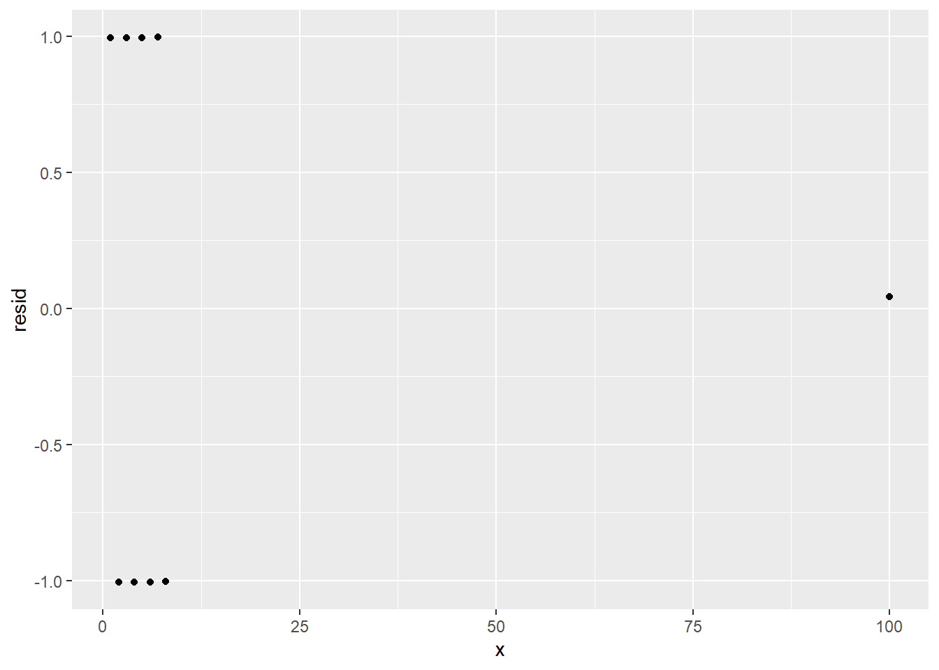

mpg_model <- lm(hwy ~ displ, data = mpg)
b <- coef(mpg_model)[1]
m <- coef(mpg_model)[2]

ggplot(mpg) +
  geom_point(aes(displ, hwy)) +
  geom_abline(intercept = 35, slope = -3) + # guessed regression line
  geom_abline(intercept = b, slope = m, color = "red") # actual regression line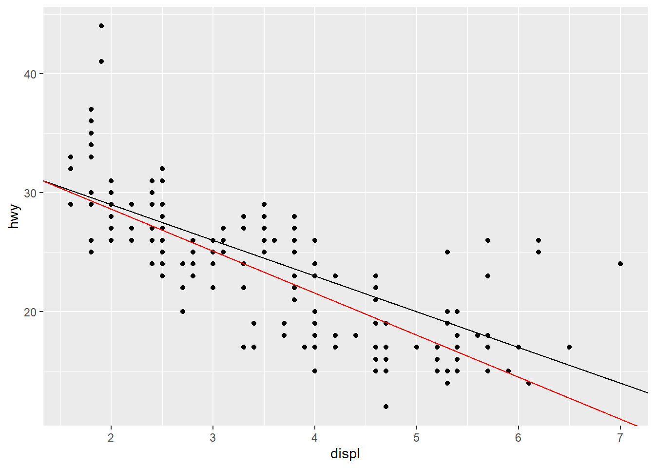

Section 4.2.1

X <- c(32.5, 29.1, 17.7, 25.1, 19.2, 26.8, 27.4, 21.1)

n <- length(X)

variance <- 1/(n - 1) * sum((X - mean(X))^2)
st_dev <- sqrt(variance)

variance

## [1] 26.29411

var(X)

## [1] 26.29411

st_dev

## [1] 5.127778

sd(X)

## [1] 5.127778

To say that the variance of X is 26.29411 means that the average squared distance between the values of X and the population mean is about 26.29411. To say that the standard deviation of X is 5.127778 means that the average distance between the values of X and the population mean is about 5.127778.

X <- rnorm(100, 50, 0.6)

X

##   [1] 49.89465 49.12142 49.64500 50.87677 49.59174 49.88390 51.28505 49.56135 50.47865 48.75779 50.52935
##  [12] 49.20785 49.54296 49.95081 50.22636 49.50480 50.20584 50.21754 49.94540 48.98020 50.34305 50.91365
##  [23] 49.84353 49.38462 51.34816 50.47381 50.43722 49.95626 49.78356 50.67631 49.74885 50.48481 50.38605
##  [34] 49.67852 49.82027 49.27375 49.27381 50.54384 49.54337 50.85396 50.73716 50.39720 50.48076 49.01576
##  [45] 50.45556 48.65065 49.63398 50.08084 49.46907 50.11526 51.11121 49.33433 49.24255 50.05063 50.10876
##  [56] 49.81916 50.98534 49.57775 49.18555 49.67709 50.02491 49.60895 51.42723 50.36917 48.88077 49.61436
##  [67] 50.11477 49.70123 49.01726 49.52215 50.29561 50.14371 51.37228 50.09824 49.14205 50.23992 50.77307
##  [78] 50.91305 48.75136 49.71756 49.99803 49.65298 49.27288 49.99510 50.09797 49.41810 49.82271 50.27230
##  [89] 49.62548 49.86603 50.43390 50.13443 48.90100 49.34616 50.52887 50.47013 49.39545 50.50800 50.69149
## [100] 50.77787

a. We know that about 70% of the values should be within 1 standard deviation (0.6) of the mean (50). We can either make this count manually by examining the list above or have R do it for us as below. We should expect about 70 of the values to fall between 49.4 and 50.6.

sum(X < 50.6 & X > 49.4)

## [1] 65

b. We know that about 95% of the values should be within 2 standard deviations (1.2) of the mean (50). We should thus expect about 95 of the values to fall between 48.8 and 51.2.

sum(X < 51.2 & X > 48.8)

## [1] 93

When $n$ is large, the difference between $\frac{1}{n}$ and $\frac{1}{n-1}$ is very small. For example, suppose $n=100000$ . The values are very close, which means we’ll get almost the same number for the biased variance and standard deviation as we do for the unbiased versions.

n <- 100000

1/n

## [1] 1e-05

1/(n - 1)

## [1] 1.00001e-05

Section 4.3.1

The model built in Section 5.1.1 which is needed for Exercises 1-5 is:

hwy = -3.53(displ) + 35.7.

The predicted value is -3.53(3.5) + 35.7 = 23.3. The actual value is 29, which gives a residual of 29 - 23.3 = 5.7.

mpg_model <- lm(hwy ~ displ, data = mpg)

mpg_w_pred_resid <- mpg %>%
  add_predictions(mpg_model) %>%
  add_residuals(mpg_model) %>%
  select(-(cyl:cty), -fl, -class)

mpg_w_pred_resid

## # A tibble: 234 x 7
##    manufacturer model      displ  year   hwy  pred  resid
##    <chr>        <chr>      <dbl> <int> <int> <dbl>  <dbl>
##  1 audi         a4           1.8  1999    29  29.3 -0.343
##  2 audi         a4           1.8  1999    29  29.3 -0.343
##  3 audi         a4           2    2008    31  28.6  2.36 
##  4 audi         a4           2    2008    30  28.6  1.36 
##  5 audi         a4           2.8  1999    26  25.8  0.188
##  6 audi         a4           2.8  1999    26  25.8  0.188
##  7 audi         a4           3.1  2008    27  24.8  2.25 
##  8 audi         a4 quattro   1.8  1999    26  29.3 -3.34 
##  9 audi         a4 quattro   1.8  1999    25  29.3 -4.34 
## 10 audi         a4 quattro   2    2008    28  28.6 -0.636
## # ... with 224 more rows
## # i Use `print(n = ...)` to see more rows

ggplot(mpg_w_pred_resid) +
  geom_point(aes(displ, resid)) +
  geom_hline(yintercept = 0)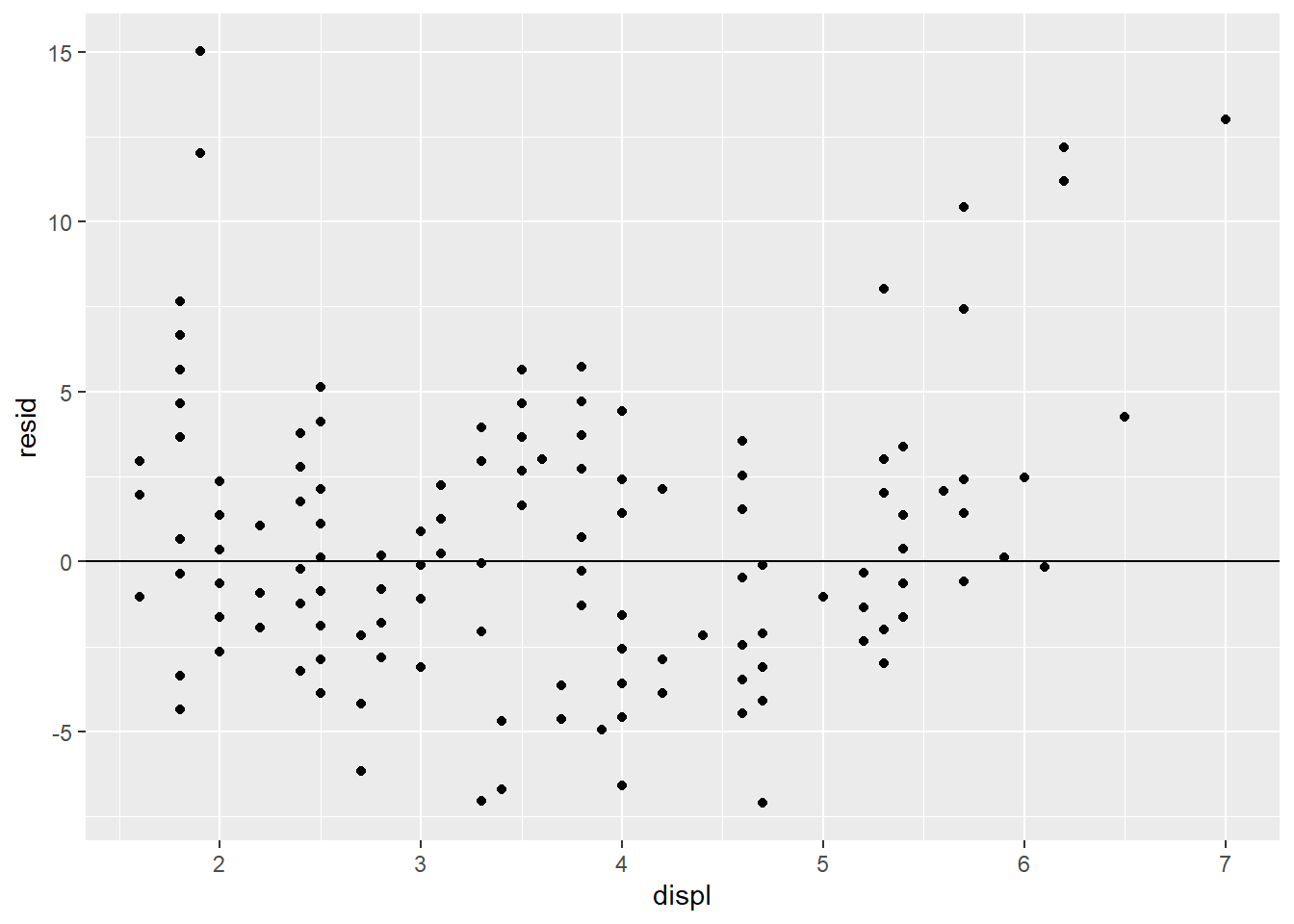

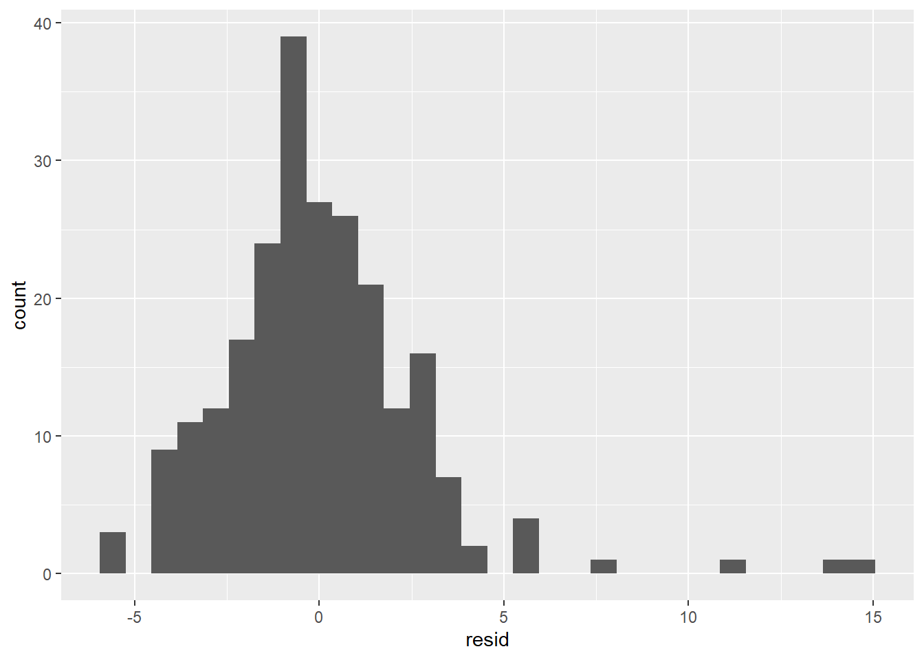
ggplot(mpg_w_pred_resid) +
  geom_histogram(aes(resid), binwidth = 1)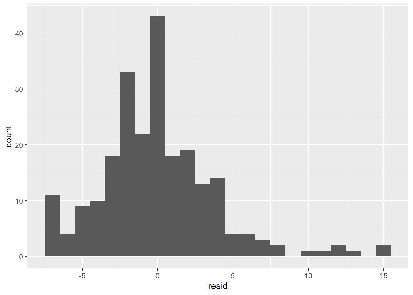

The residuals don’t exhibit a very strong pattern. However, it does seem that the model significantly under-predicts for cars with very small or very large engines, which means that for these cars, engine size alone is not a good predictor of highway fuel efficiency. There must be other variables that explain why the hwy values are so high. (Small-engine cars include hybrids, which get very high gas mileage. Among large-engine cars are two-seaters, which get surprisingly high gas mileage for their engine size because they are light weight and very aerodynamic.)

The residual distribution is somewhat normal, although it seems right-skewed rather than symmetrical. The reason is the same as given in the last paragraph: There are some large positive residuals, which are explained by cars for which the model significantly under-predicts the hwy value. There is also a spike at the far left, indicating that there are also cars for which the model significantly over-predicts.

Based on these residual visualizations, we can say that a linear regression model is appropriate, but it’s clear that there are other variables that would be needed to predict hwy better, such as class. We’ll see how to add extra predictors to a model in Section 4.6.

The residuals in (c) appear to exhibit less of a pattern than the others, which means that it is most indicative of a good linear model.
The residuals do not exhibit a pattern and the distribution is roughly normal, meaning that the data is appropriately modeled by a linear regression model.

library(readr)
height_weight <- read_csv("height-weight.csv")

height_model <- lm(`Weight(Pounds)` ~ `Height(Inches)`, data = height_weight)

height_weight_w_resid <- height_weight %>%
  add_residuals(height_model)

ggplot(height_weight_w_resid) +
  geom_point(aes(`Height(Inches)`, resid)) +
  geom_hline(yintercept = 0)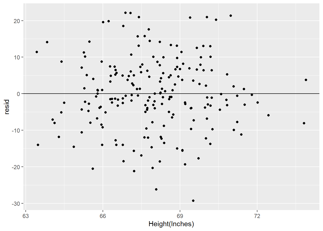

ggplot(height_weight_w_resid) +
  geom_histogram(aes(resid), binwidth = 1.5)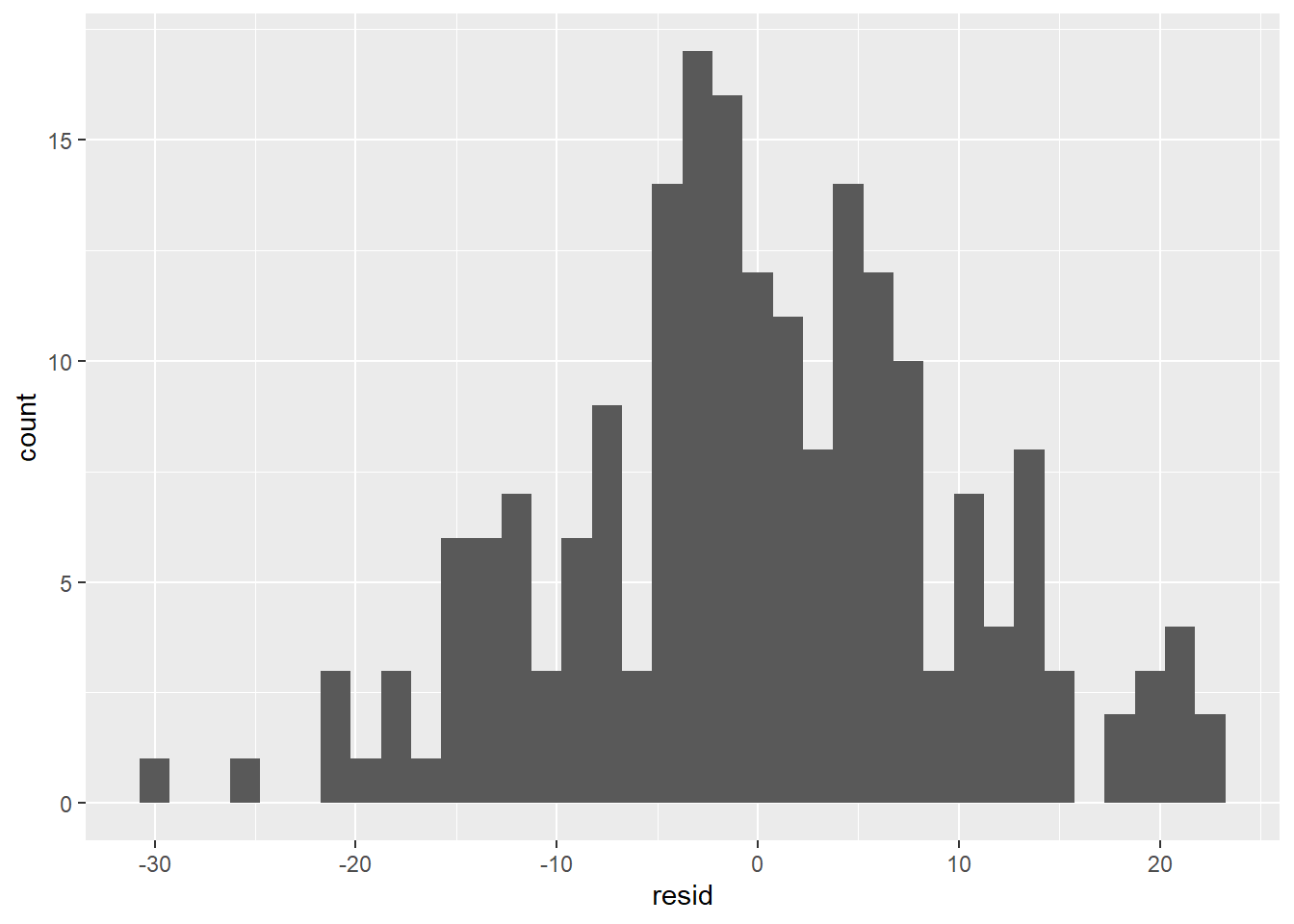

Section 4.4.1

The model we need for Exercises 1-2 is:

mpg_model <- lm(hwy ~ displ, data = mpg)

We can run the model’s summary to see that the RSE is 3.836.

summary(mpg_model)

## 
## Call:
## lm(formula = hwy ~ displ, data = mpg)
## 
## Residuals:
##     Min      1Q  Median      3Q     Max 
## -7.1039 -2.1646 -0.2242  2.0589 15.0105 
## 
## Coefficients:
##             Estimate Std. Error t value Pr(>|t|)    
## (Intercept)  35.6977     0.7204   49.55   <2e-16 ***
## displ        -3.5306     0.1945  -18.15   <2e-16 ***
## ---
## Signif. codes:  0 '***' 0.001 '**' 0.01 '*' 0.05 '.' 0.1 ' ' 1
## 
## Residual standard error: 3.836 on 232 degrees of freedom
## Multiple R-squared:  0.5868, Adjusted R-squared:  0.585 
## F-statistic: 329.5 on 1 and 232 DF,  p-value: < 2.2e-16

a. 3.836
b. 7.672 (which equals twice the RSE)

By examining the plot below, we see there are 8 points outside the blue lines which make up the 95% confidence band. We also know there are 234 data points total in mpg. Thus, the band contains 226 out of 234 data points, which is about 96.6%. This is close to the expected 95%.

mpg_coefs <- coef(mpg_model)
b <- mpg_coefs[1]
m <- mpg_coefs[2]

ggplot(mpg) +
  geom_point(aes(displ, hwy)) +
  geom_abline(slope = m, intercept = b) +
  geom_abline(slope = m, intercept = b + 7.672, color = "blue") +
  geom_abline(slope = m, intercept = b - 7.672, color = "blue")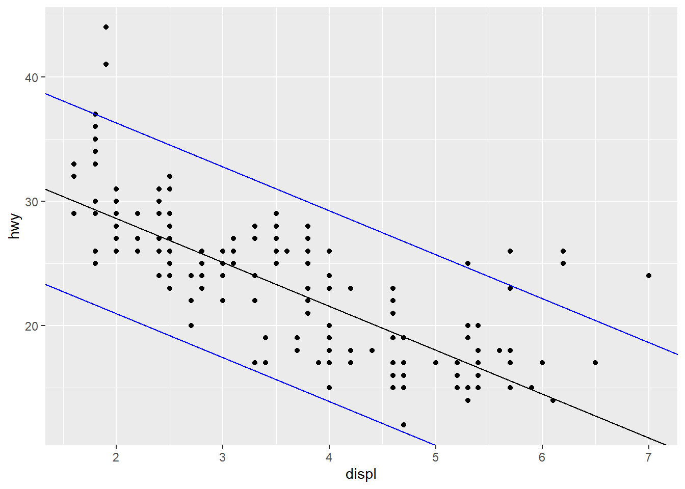

The RSE of the model is 0.7634, which means that we can be 95% confident that the prediction is within 1.5268 of the true value. However, the residual distribution was not very normal-looking, and there are only 10 data points. Further, the RSE was computed with only 8 degrees of freedom, which is extremely low. Therefore, we should not put too much trust in this confidence interval.

sim1a <- readr::read_csv("https://raw.githubusercontent.com/jafox11/MS282/main/sim1_a.csv")

sim1a_model <- lm(y ~ x, data = sim1a)

summary(sim1a_model)

## 
## Call:
## lm(formula = y ~ x, data = sim1a)
## 
## Residuals:
##     Min      1Q  Median      3Q     Max 
## -1.1206 -0.4750  0.1561  0.5620  0.9511 
## 
## Coefficients:
##             Estimate Std. Error t value Pr(>|t|)    
## (Intercept)  6.36737    0.52153   12.21 1.88e-06 ***
## x            1.45886    0.08405   17.36 1.24e-07 ***
## ---
## Signif. codes:  0 '***' 0.001 '**' 0.01 '*' 0.05 '.' 0.1 ' ' 1
## 
## Residual standard error: 0.7634 on 8 degrees of freedom
## Multiple R-squared:  0.9741, Adjusted R-squared:  0.9709 
## F-statistic: 301.3 on 1 and 8 DF,  p-value: 1.237e-07

Section 4.5.1

The multiple R² value is 0.5868, which means that the model can explain about 58.68% of the variance in the hwy variable. The rest of the variance is explained by randomness or other variables not used by the model. The adjusted R² value is 0.585, which can be interpreted in the same way: The model explains about 58.5% of the variance in hwy. The difference is that multiple R² values are biased, whereas adjust R² values are not.

mpg_model <- lm(hwy ~ displ, data = mpg)

summary(mpg_model)

## 
## Call:
## lm(formula = hwy ~ displ, data = mpg)
## 
## Residuals:
##     Min      1Q  Median      3Q     Max 
## -7.1039 -2.1646 -0.2242  2.0589 15.0105 
## 
## Coefficients:
##             Estimate Std. Error t value Pr(>|t|)    
## (Intercept)  35.6977     0.7204   49.55   <2e-16 ***
## displ        -3.5306     0.1945  -18.15   <2e-16 ***
## ---
## Signif. codes:  0 '***' 0.001 '**' 0.01 '*' 0.05 '.' 0.1 ' ' 1
## 
## Residual standard error: 3.836 on 232 degrees of freedom
## Multiple R-squared:  0.5868, Adjusted R-squared:  0.585 
## F-statistic: 329.5 on 1 and 232 DF,  p-value: < 2.2e-16

The R² value is 0.999, which would indicate that the model can explain almost 100% of the variance in the y variable. However, the residuals exhibit a very obvious pattern, which means that the model is still missing an important relationship between x and y, despite the very high R² value.

df <- tibble(
  x = c(1, 2, 3, 4, 5, 6, 7, 8, 100),
  y = c(2, 1, 4, 3, 6, 5, 8, 7, 100)
)

df_model <- lm(y ~ x, data = df)

summary(df_model)

## 
## Call:
## lm(formula = y ~ x, data = df)
## 
## Residuals:
##      Min       1Q   Median       3Q      Max 
## -1.00644 -1.00447  0.04167  0.99406  0.99602 
## 
## Coefficients:
##             Estimate Std. Error t value Pr(>|t|)    
## (Intercept) 0.007418   0.398710   0.019    0.986    
## x           0.999509   0.011841  84.410 8.62e-12 ***
## ---
## Signif. codes:  0 '***' 0.001 '**' 0.01 '*' 0.05 '.' 0.1 ' ' 1
## 
## Residual standard error: 1.069 on 7 degrees of freedom
## Multiple R-squared:  0.999,  Adjusted R-squared:  0.9989 
## F-statistic:  7125 on 1 and 7 DF,  p-value: 8.624e-12

df_w_resid <- df %>%
  add_residuals(df_model)

ggplot(df_w_resid) +
  geom_point(aes(x, resid))

For an R² value to be negative, the ratio $\frac{\textrm{MSR}}{\textrm{variance}}$ would have to be greater than 1. This happens when the MSR is greater than the variance. When this is the case, the actual values of the response variable are, on average, closer to the mean response value than they are to the model’s predicted response values. In other words, the R² value will be negative when the model does a worse job making predictions than one which would just predict the mean.
Statement (2) is more meaningful. Knowing the RSE without knowing anything about the magnitude of the response values doesn’t tell us anything; we would have no frame of reference to know whether an RSE of 2.25 should be considered high or low. The R² value, on the other hand, does not need a frame of reference. To say that the model can explain 78% of the variation is meaningful even if we don’t know anything about the data set.

Section 4.6.1

The coefficient (slope) is -3.5306, the standard error is 0.1945, the t-statistic is -18.15, and the p-value is $2\times 10^{-16}$ (which is the smallest non-zero number R can display).

mpg_model <- lm(hwy ~ displ, data = mpg)

summary(mpg_model)

## 
## Call:
## lm(formula = hwy ~ displ, data = mpg)
## 
## Residuals:
##     Min      1Q  Median      3Q     Max 
## -7.1039 -2.1646 -0.2242  2.0589 15.0105 
## 
## Coefficients:
##             Estimate Std. Error t value Pr(>|t|)    
## (Intercept)  35.6977     0.7204   49.55   <2e-16 ***
## displ        -3.5306     0.1945  -18.15   <2e-16 ***
## ---
## Signif. codes:  0 '***' 0.001 '**' 0.01 '*' 0.05 '.' 0.1 ' ' 1
## 
## Residual standard error: 3.836 on 232 degrees of freedom
## Multiple R-squared:  0.5868, Adjusted R-squared:  0.585 
## F-statistic: 329.5 on 1 and 232 DF,  p-value: < 2.2e-16

To say that the coefficient is -3.5306 means that for every increase of 1 liter in the displ variable, the highway fuel efficiency drops by about 3.5306 miles per gallon.

To say that the standard error is 0.1945 means that on average, we would estimate a deviation of about 0.1945 from the true coefficient value when estimating the value of the coefficient.

To say that the t-statistic is -18.15 means that the value of our coefficient is about 18.15 standard errors below 0.

To say that the p-value is $2\times 10^{-16}$ means that assuming the true value of our coefficient is 0, the probability of getting a value of -3.5306 or less as the result of statistical randomness is $2\times 10^{-16}$ .

Yes, it does since the p-value is less than 0.05.
The intercept is about 35.7 and it has a very small p-value, so it’s statistically significant. However, it does not have a meaningful interpretation in this context because it would be the highway fuel efficiency of a car with a 0-liter engine.
For part (a), we should make it so that the coefficient of w is a large positive number and/or the standard error for w is small. We can guarantee this by making the relationship between w and z highly linear with a large positive slope.

For part (b), we can replicate what we did for part (a), but make the slope a large negative number.

For part (c), we should make it so that the coefficient of y is near 0 and/or there is no linear relationship between y and z.

The following data set is one such example.

df <- tibble(
  w = c(1, 2, 3, 4, 5, 6, 7, 8, 9, 10),
  x = c(10, 9, 8, 7, 6, 5, 4, 3, 2, 1),
  y = c(1, 2, 3, 4, 5, 5, 4, 3, 2, 1),
  z = c(5, 10, 15, 20, 25, 30, 35, 40, 45, 50)
)

df_model_w <- lm(z ~ w, data = df)

summary(df_model_w)

## 
## Call:
## lm(formula = z ~ w, data = df)
## 
## Residuals:
##        Min         1Q     Median         3Q        Max 
## -4.756e-15 -1.193e-15 -2.021e-16  1.623e-15  3.315e-15 
## 
## Coefficients:
##               Estimate Std. Error    t value Pr(>|t|)    
## (Intercept) -4.494e-15  1.736e-15 -2.588e+00   0.0322 *  
## w            5.000e+00  2.798e-16  1.787e+16   <2e-16 ***
## ---
## Signif. codes:  0 '***' 0.001 '**' 0.01 '*' 0.05 '.' 0.1 ' ' 1
## 
## Residual standard error: 2.541e-15 on 8 degrees of freedom
## Multiple R-squared:      1,  Adjusted R-squared:      1 
## F-statistic: 3.193e+32 on 1 and 8 DF,  p-value: < 2.2e-16

df_model_x <- lm(z ~ x, data = df)

summary(df_model_x)

## 
## Call:
## lm(formula = z ~ x, data = df)
## 
## Residuals:
##        Min         1Q     Median         3Q        Max 
## -9.425e-15 -2.428e-16  7.752e-16  1.120e-15  5.908e-15 
## 
## Coefficients:
##               Estimate Std. Error    t value Pr(>|t|)    
## (Intercept)  5.500e+01  2.766e-15  1.988e+16   <2e-16 ***
## x           -5.000e+00  4.458e-16 -1.122e+16   <2e-16 ***
## ---
## Signif. codes:  0 '***' 0.001 '**' 0.01 '*' 0.05 '.' 0.1 ' ' 1
## 
## Residual standard error: 4.049e-15 on 8 degrees of freedom
## Multiple R-squared:      1,  Adjusted R-squared:      1 
## F-statistic: 1.258e+32 on 1 and 8 DF,  p-value: < 2.2e-16

df_model_y <- lm(z ~ y, data = df)

summary(df_model_y)

## 
## Call:
## lm(formula = z ~ y, data = df)
## 
## Residuals:
##    Min     1Q Median     3Q    Max 
## -22.50 -11.25   0.00  11.25  22.50 
## 
## Coefficients:
##              Estimate Std. Error t value Pr(>|t|)  
## (Intercept) 2.750e+01  1.191e+01   2.309   0.0497 *
## y           1.589e-15  3.590e+00   0.000   1.0000  
## ---
## Signif. codes:  0 '***' 0.001 '**' 0.01 '*' 0.05 '.' 0.1 ' ' 1
## 
## Residual standard error: 16.06 on 8 degrees of freedom
## Multiple R-squared:  4.284e-32,  Adjusted R-squared:  -0.125 
## F-statistic: 3.427e-31 on 1 and 8 DF,  p-value: 1

1. There are two things wrong with this statement. First, the p-value tells you the probability of obtaining a slope whose absolute value is 3.1 or greater. Second, the p-value is a probability calculated under the assumption that the null hypothesis is true. The correct way to word this statement is, “Assuming that E has no significant impact on R, the probability of obtaining a slope whose absolute value is 3.1 or greater is 23%.”
2. Getting a p-value above the 0.05 threshold means that there is not enough evidence to reject the null hypothesis, which is not the same as accepting it. (By analogy, you might not believe there’s enough evidence to disbelieve is Santa Claus, but that doesn’t necessarily mean you have to believe in him.) The correct way to word the statement is, “Since the p-value is above the 0.05 threshold, we cannot reject the null hypothesis, which means we don’t have enough evidence to conclude that E has a significant impact on R.”
1. To reject the null hypothesis is to say that we have enough evidence to conclude that the intercept is not 0. It doesn’t necessarily mean that the true value is 77.09, though.
2. The multiple R² is 0.0003758, which means our model can only explain about 0.038% of the variation. Even worse, the adjusted R² value is -0.05516. A negative R² value means that we’d be better off just using the mean of the exam scores as our prediction rather than using the model to make a prediction. In other words, our model is useless, so despite their low p-values, we shouldn’t attribute any real meaning to the coefficients. This model would not make it past the post-assessment stage, so we shouldn’t be trying to interpret anything with it.
Since the RSE is 10.34, the endpoints of our 95% CI are +/- 20.68. This means that if our model predicts an exam score of 60%, then there’s a 95% chance that the actual score is somewhere between about 40% and 80%. That’s not very impressive! The large RSE is more reason to not move on to the interpretation stage.

Section 4.7.1

library(readr)
car_prices <- read_csv("car_prices.csv")

car_prices_model <- lm(price ~ `highway-mpg`, data = car_prices)

The coefficient is -821.50, which means that for each additional mile per gallon of highway fuel efficiency, the selling price drops by about $821.50. The p-value is extremely small, meaning that this coefficient is statistically significant. The conclusion we can draw is that cars with better fuel efficiency are cheaper. This might seem surprising since it should be the case that high fuel efficiency adds value to a car rather than subtracts from it.

summary(car_prices_model)

## 
## Call:
## lm(formula = price ~ `highway-mpg`, data = car_prices)
## 
## Residuals:
##    Min     1Q Median     3Q    Max 
##  -8679  -3418  -1136   1063  20938 
## 
## Coefficients:
##               Estimate Std. Error t value Pr(>|t|)    
## (Intercept)   38450.00    1849.66   20.79   <2e-16 ***
## `highway-mpg`  -821.50      58.84  -13.96   <2e-16 ***
## ---
## Signif. codes:  0 '***' 0.001 '**' 0.01 '*' 0.05 '.' 0.1 ' ' 1
## 
## Residual standard error: 5671 on 197 degrees of freedom
## Multiple R-squared:  0.4973, Adjusted R-squared:  0.4948 
## F-statistic: 194.9 on 1 and 197 DF,  p-value: < 2.2e-16

Both curb-weight and horsepower might be confounding variables since they are correlated with both price and highway-mpg. As curb-weight and horsepower increase, price generally increases, but highway-mpg generally decreases.

car_prices_model2 <- lm(price ~ `highway-mpg` + `curb-weight` + horsepower, data = car_prices)

The new coefficient of highway-mpg is about 183.6, meaning that for a given curb weight and horsepower, each additional mpg of highway fuel efficiency adds about $183.60 to the car’s value. The p-value is 0.0157, which is below the 0.05 cutoff, meaning that the coefficient is statistically significant.

summary(car_prices_model2)

## 
## Call:
## lm(formula = price ~ `highway-mpg` + `curb-weight` + horsepower, 
##     data = car_prices)
## 
## Residuals:
##     Min      1Q  Median      3Q     Max 
## -9002.2 -2021.6    53.3  1617.2 15977.7 
## 
## Coefficients:
##                 Estimate Std. Error t value Pr(>|t|)    
## (Intercept)   -2.624e+04  4.324e+03  -6.069 6.59e-09 ***
## `highway-mpg`  1.836e+02  7.531e+01   2.438   0.0157 *  
## `curb-weight`  9.014e+00  9.034e-01   9.978  < 2e-16 ***
## horsepower     1.046e+02  1.278e+01   8.183 3.52e-14 ***
## ---
## Signif. codes:  0 '***' 0.001 '**' 0.01 '*' 0.05 '.' 0.1 ' ' 1
## 
## Residual standard error: 3786 on 195 degrees of freedom
## Multiple R-squared:  0.7782, Adjusted R-squared:  0.7748 
## F-statistic: 228.1 on 3 and 195 DF,  p-value: < 2.2e-16

The conclusion from Exercise 3 is an example of omitted variable bias because it is a misleading statement that is due to the omission of relevant variables as predictors.
One example of omitted variable bias might be to say that since the number of reported sunburns seems to increase when an ice cream stand sells more ice cream, that it must be the case that ice cream causes sun burns. The omitted variable here, though, would be the air temperature. As temperature goes up, so does the amount of ice cream sold and the number of reported sun burns.

Section 4.8.1

The model is given by:

diamonds_model_4 <- lm(price ~ carat + depth + table, data = diamonds)

The summary below shows that the multiple and adusted R² values are both 0.8537. If more decimal places could be displayed, we’d eventually see a difference, but they’re the same through four decimal places. This is because diamonds has 53,940 observations, whereas the number of degrees of freedom is 53,936. The values of the fractions $\frac{1}{53940}$ and $\frac{1}{53936}$ are so close, the amount of bias built into the multiple R² won’t be noticeable, and this leads to nearly equal multiple and adjusted R² values.

summary(diamonds_model_4)

## 
## Call:
## lm(formula = price ~ carat + depth + table, data = diamonds)
## 
## Residuals:
##      Min       1Q   Median       3Q      Max 
## -18288.0   -785.9    -33.2    527.2  12486.7 
## 
## Coefficients:
##              Estimate Std. Error t value Pr(>|t|)    
## (Intercept) 13003.441    390.918   33.26   <2e-16 ***
## carat        7858.771     14.151  555.36   <2e-16 ***
## depth        -151.236      4.820  -31.38   <2e-16 ***
## table        -104.473      3.141  -33.26   <2e-16 ***
## ---
## Signif. codes:  0 '***' 0.001 '**' 0.01 '*' 0.05 '.' 0.1 ' ' 1
## 
## Residual standard error: 1526 on 53936 degrees of freedom
## Multiple R-squared:  0.8537, Adjusted R-squared:  0.8537 
## F-statistic: 1.049e+05 on 3 and 53936 DF,  p-value: < 2.2e-16

The coefficient of carat means that with each addition carat added to the weight of a diamond, the price goes up by about $7,858. The coefficient of depth means that with each additional percentage point added to the depth, the price drops by about $151. The coefficient of table means that with each unit added to the table value, the price drops by about $104.
The p-value of each coefficient is extremely low, meaning that the coefficient values are statistically significant.
The residuals appear to be approximately normal.

diamonds_w_resid <- diamonds %>%
  add_residuals(diamonds_model_4)

ggplot(diamonds_w_resid) +
  geom_histogram(aes(resid), binwidth = 750)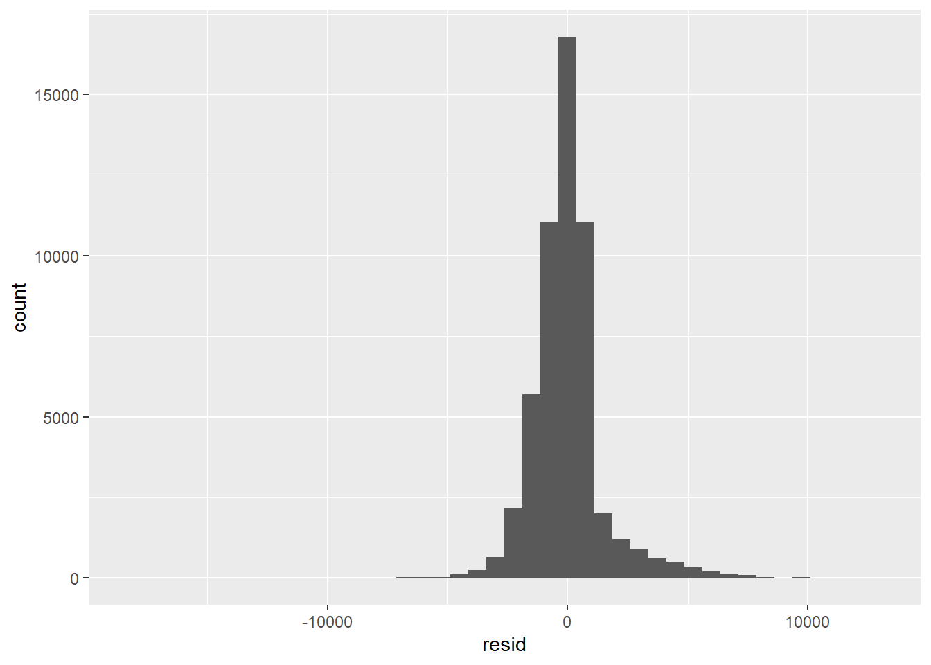

Since the residuals are normally distributed, we can state the 95% CI. The summary above shows that the RSE of the model is 1526. This means that we can be 95% confident that a given prediction is within $3,052 of the actual price.

delay_model <- lm(arr_delay ~ dep_delay + air_time + distance, data = flights)

delay_model

## 
## Call:
## lm(formula = arr_delay ~ dep_delay + air_time + distance, data = flights)
## 
## Coefficients:
## (Intercept)    dep_delay     air_time     distance  
##   -15.91942      1.01957      0.68698     -0.08919

The air_time and distance coefficients seem contradictory. You wouldn’t expect them to affect the arrival delay in opposite ways, but the reason is that these two variables are likely highly correlated. So the counter-intuitive coefficients are probably side-effects of collinearity.
The correlation coefficient between air_time and distance is almost 1, which means these two variables are highly correlated.

arr_delay_predictors <- flights %>%
  select(dep_delay, air_time, distance) %>%
  filter(!is.na(dep_delay) & !is.na(air_time) & !is.na(distance))

cor(arr_delay_predictors)

##             dep_delay    air_time   distance
## dep_delay  1.00000000 -0.02240508 -0.0216809
## air_time  -0.02240508  1.00000000  0.9906496
## distance  -0.02168090  0.99064965  1.0000000

We’ll keep air_time and delete distance. Previously, air_time had a positive coefficient, but in the new non-collinear model, air_time has a negative coefficient. A negative coefficient makes more sense because the longer the flight is, the more time you have to make up for a departure delay, thus decreasing the arrival delay.

delay_model2 <- lm(arr_delay ~ dep_delay + air_time, data = flights)

delay_model2

## 
## Call:
## lm(formula = arr_delay ~ dep_delay + air_time, data = flights)
## 
## Coefficients:
## (Intercept)    dep_delay     air_time  
##   -4.831805     1.018723    -0.007055

Comparing the summaries below, we see that the R² value increases a very little bit after the outliers are removed. Also, the coefficient of x increases slightly. In this case, removing the outliers didn’t make much of a difference, probably because there are very few of them compared to the size of the data set.

outliers_present <- lm(price ~ x, data = diamonds)

summary(outliers_present)

## 
## Call:
## lm(formula = price ~ x, data = diamonds)
## 
## Residuals:
##    Min     1Q Median     3Q    Max 
##  -8426  -1264   -185    973  32128 
## 
## Coefficients:
##               Estimate Std. Error t value Pr(>|t|)    
## (Intercept) -14094.056     41.732  -337.7   <2e-16 ***
## x             3145.413      7.146   440.2   <2e-16 ***
## ---
## Signif. codes:  0 '***' 0.001 '**' 0.01 '*' 0.05 '.' 0.1 ' ' 1
## 
## Residual standard error: 1862 on 53938 degrees of freedom
## Multiple R-squared:  0.7822, Adjusted R-squared:  0.7822 
## F-statistic: 1.937e+05 on 1 and 53938 DF,  p-value: < 2.2e-16

diamonds2 <- diamonds %>%
  filter(x > 3)
    
outliers_removed <- lm(price ~ x, diamonds2)

summary(outliers_removed)

## 
## Call:
## lm(formula = price ~ x, data = diamonds2)
## 
## Residuals:
##     Min      1Q  Median      3Q     Max 
## -8476.1 -1265.4  -178.1   990.5 12087.7 
## 
## Coefficients:
##               Estimate Std. Error t value Pr(>|t|)    
## (Intercept) -14184.869     41.332  -343.2   <2e-16 ***
## x             3160.674      7.077   446.6   <2e-16 ***
## ---
## Signif. codes:  0 '***' 0.001 '**' 0.01 '*' 0.05 '.' 0.1 ' ' 1
## 
## Residual standard error: 1840 on 53930 degrees of freedom
## Multiple R-squared:  0.7872, Adjusted R-squared:  0.7872 
## F-statistic: 1.995e+05 on 1 and 53930 DF,  p-value: < 2.2e-16

In this case, it would not make sense to impute the mean value into the missing values of dep_delay since the NAs in this column are meaningful; they indicate a cancelled flight. To give them a value would cause us to pretend that these flights weren’t cancelled. In this case, it would be better to filter our the rows with missing values in the dep_delay column.

Section 4.9.1

The model is hwy = 24.8 + 3.498(classcompact) + 2.493(classmidsize) - 2.436(classminivan) - 7.921(classpickup) + 3.343(classsubcompact) - 6.671(classsuv)

class_model <- lm(hwy ~ class, data = mpg)

class_model

## 
## Call:
## lm(formula = hwy ~ class, data = mpg)
## 
## Coefficients:
##     (Intercept)     classcompact     classmidsize     classminivan      classpickup  classsubcompact  
##          24.800            3.498            2.493           -2.436           -7.921            3.343  
##        classsuv  
##          -6.671

1. Use 1 for classsuv and 0 for the others. This gives 18.129.
2. Use 1 for classsubcompact and 0 for the others. This gives 28.143.
3. Since there is no class2seater variable, we use 0 for all the variables. This gives 24.8.
The R² value is 0.6879, which means the model can explain about 69% of the variation in the hwy variable. This is pretty good. The RSE is 3.37, which means we can be about 70% confident that any prediction is within 3.37 of the actual hwy value and 95% confident that any prediction is within 6.74 of the actual hwy value. This is also moderately good, given the sizes of the hwy values.

summary(class_model)

## 
## Call:
## lm(formula = hwy ~ class, data = mpg)
## 
## Residuals:
##     Min      1Q  Median      3Q     Max 
## -8.1429 -1.8788 -0.2927  1.1803 15.8571 
## 
## Coefficients:
##                 Estimate Std. Error t value Pr(>|t|)    
## (Intercept)       24.800      1.507  16.454  < 2e-16 ***
## classcompact       3.498      1.585   2.206   0.0284 *  
## classmidsize       2.493      1.596   1.561   0.1198    
## classminivan      -2.436      1.818  -1.340   0.1815    
## classpickup       -7.921      1.617  -4.898 1.84e-06 ***
## classsubcompact    3.343      1.611   2.075   0.0391 *  
## classsuv          -6.671      1.567  -4.258 3.03e-05 ***
## ---
## Signif. codes:  0 '***' 0.001 '**' 0.01 '*' 0.05 '.' 0.1 ' ' 1
## 
## Residual standard error: 3.37 on 227 degrees of freedom
## Multiple R-squared:  0.6879, Adjusted R-squared:  0.6797 
## F-statistic: 83.39 on 6 and 227 DF,  p-value: < 2.2e-16

First, the R² value is 0.4836. This isn’t great, but it’s not terrible. We can’t expect big R² values for this simple regression model with a binary predictor, since something as unpredictable as life expectancy can’t be explained by a single yes/no variable. Regardless, the coefficient of the Western Europe value is -1.1235, which means that the average life expectancy in Western Europe is about 1.1235 years less than the average life expectancy in Northern Europe. The p-value of this coefficient is 0.00831, which is less than the 0.05 cutoff. This indicates that the 1.1235-year life expectancy difference is significant.

library(readr)
Europe <- read_csv("Europe.csv")

Europe_model <- lm(Life_Expectancy ~ Region, data = Europe)

summary(Europe_model)

## 
## Call:
## lm(formula = Life_Expectancy ~ Region, data = Europe)
## 
## Residuals:
##      Min       1Q   Median       3Q      Max 
## -1.02520 -0.51150 -0.04321  0.51626  0.75192 
## 
## Coefficients:
##                      Estimate Std. Error t value Pr(>|t|)    
## (Intercept)           82.5764     0.2569 321.475  < 2e-16 ***
## RegionWestern Europe  -1.1235     0.3501  -3.209  0.00831 ** 
## ---
## Signif. codes:  0 '***' 0.001 '**' 0.01 '*' 0.05 '.' 0.1 ' ' 1
## 
## Residual standard error: 0.6292 on 11 degrees of freedom
## Multiple R-squared:  0.4836, Adjusted R-squared:  0.4366 
## F-statistic:  10.3 on 1 and 11 DF,  p-value: 0.008314

1. The long right tail of the histogram means that there are a significant number of cars with large positive residuals, which means that the model underpredicts the value of hwy. As we have seen, this must be due to the 2seater and compact classes, which have cars that get much better gas mileage than would be predicted.

mpg_model <- lm(hwy ~ displ, data = mpg)

mpg_model_w_resid <- mpg %>%
  add_residuals(mpg_model)

ggplot(mpg_model_w_resid) +
  geom_histogram(aes(resid))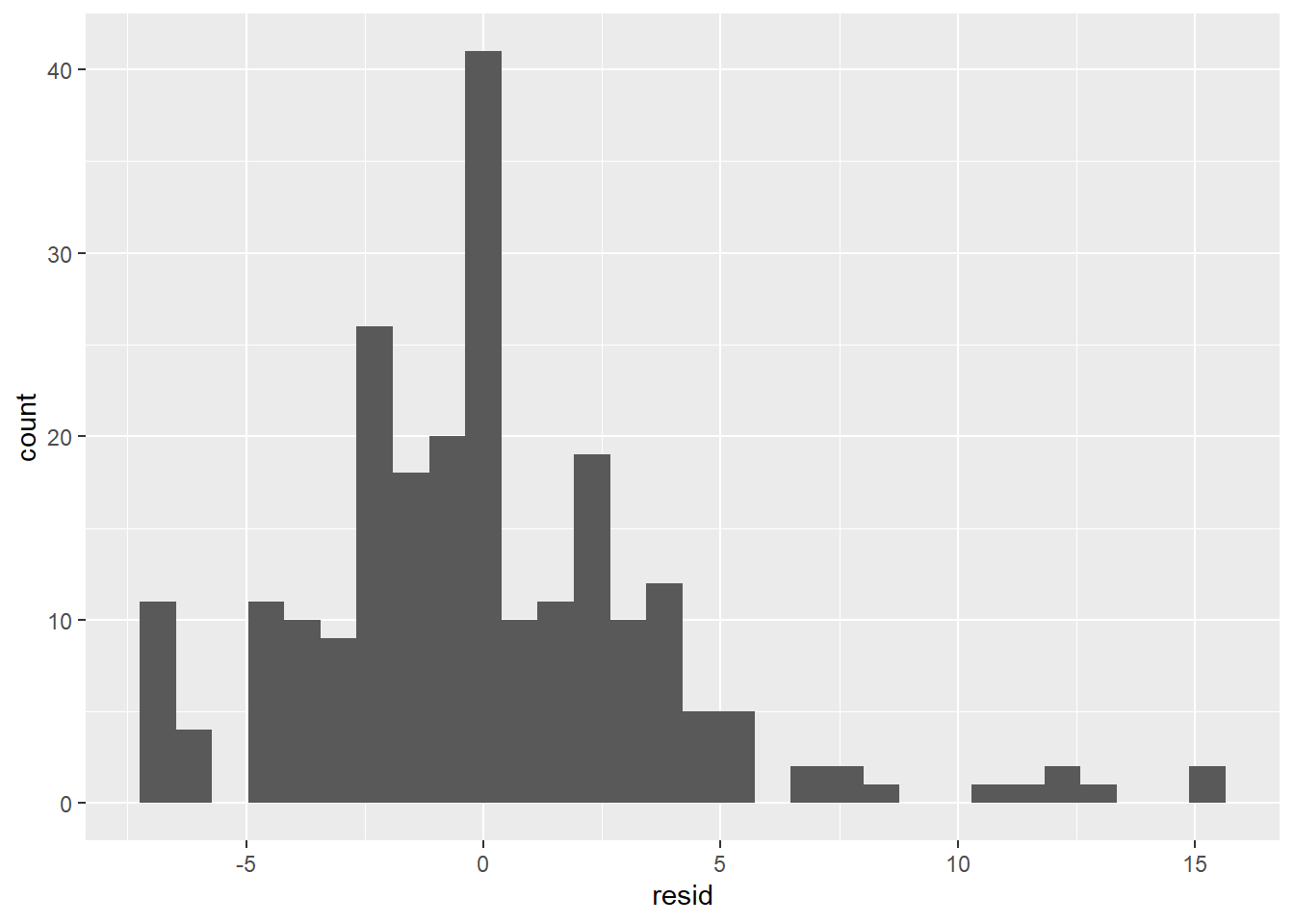

b.

mpg_model2 <- lm(hwy ~ displ + class, data = mpg)

c. The new histogram looks a little more normal. We see few cars in the right tail, indicating that by controlling for `class`, we were able to partly explain the under-predictions the original model had made.

mpg_w_resid2 <- mpg %>%
  add_residuals(mpg_model2)

ggplot(mpg_w_resid2) +
  geom_histogram(aes(resid))