5 Analysis
- Answers to the research questions
- Different methods considered
- Competing approaches
- Justifications
5.1 Research Questions
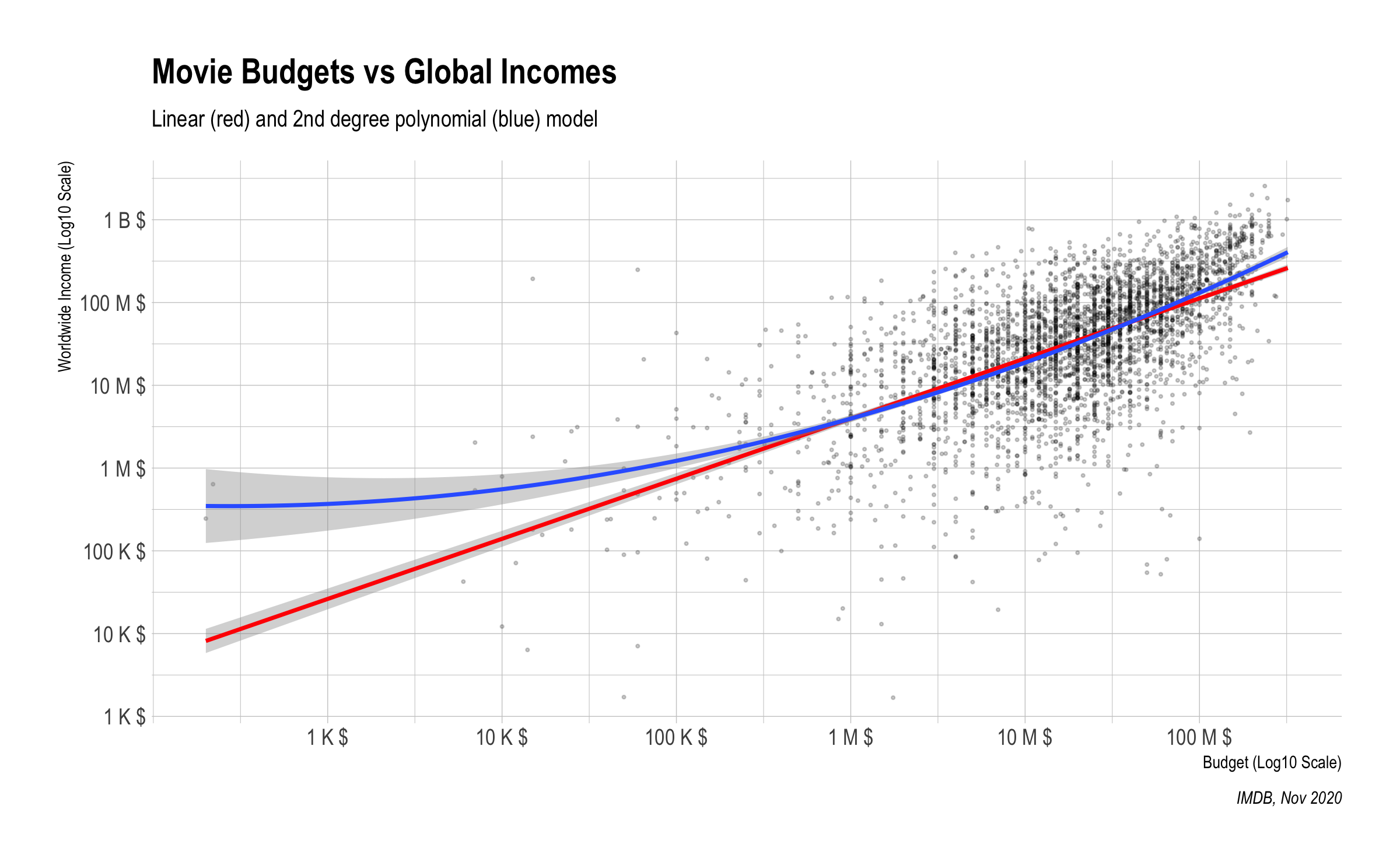
Do budgets positively correlate with profits?
During the exploratory data analysis, the clear correlation between budget and income was observed. For modelling of that relation 4 different models were used and compared to their adj.r.squared value. As expected, the linear model was best when both budget and income was at logarithmic scale.
#> # A tibble: 4 x 3
#>   model                         r_squared adj_r_squraed
#>   <chr>                             <dbl>         <dbl>
#> 1 Linear Model                      0.405         0.405
#> 2 Polynomial Model (2nd degree)     0.416         0.415
#> 3 Polynomial Model (3rd degree)     0.416         0.415
#> 4 Linear Model (Log)                0.389         0.389
#>
#> Call:
#> lm(formula = profit ~ poly(budget, degree = 2), data = drop_na(movies_df,
#> budget))
#>
#> Residuals:
#> Min 1Q Median 3Q Max
#> -6.96e+08 -4.11e+07 -2.19e+07 1.38e+07 1.89e+09
#>
#> Coefficients:
#> Estimate Std. Error t value Pr(>|t|)
#> (Intercept) 9.74e+07 2.12e+06 45.96 <2e-16 ***
#> poly(budget, degree = 2)1 6.53e+09 1.29e+08 50.67 <2e-16 ***
#> poly(budget, degree = 2)2 1.05e+09 1.29e+08 8.11 7e-16 ***
#> ---
#> Signif. codes: 0 '***' 0.001 '**' 0.01 '*' 0.05 '.' 0.1 ' ' 1
#>
#> Residual standard error: 1.29e+08 on 3701 degrees of freedom
#> Multiple R-squared: 0.416, Adjusted R-squared: 0.415
#> F-statistic: 1.32e+03 on 2 and 3701 DF, p-value: <2e-16According to predicted best model (Polynomial Model (2nd degree)), each unit increase of the budget significantly (p < 2e-16) increase the profit variable. So, budgets positively correlate with profits. While, the polynomial model is slightly better according the adjusted r squared value (explains %1 more of the outcome variability compared to linear model), the linear model is preferred for the rest of the analysis as it is more easier to interpret and comment. The graph below also shows that both model has similar trend in the majority of the data.
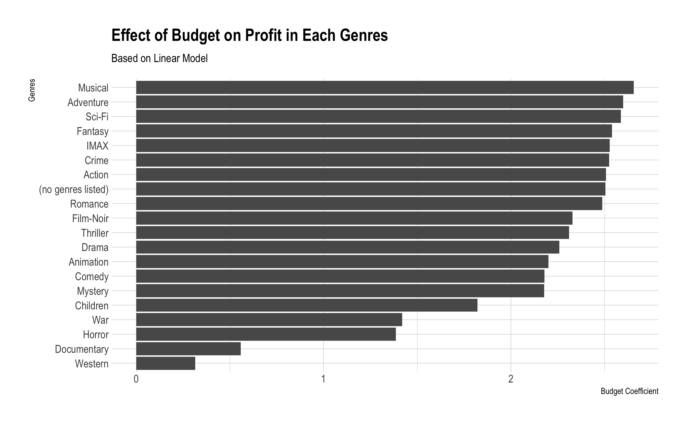
Does this prediction change regarding the movie genre?
To understand the relation between budget and profit in different genres, same linear modelling was applied in each genres seperately. The table below shows the coefficients of the budget in different genres. Except documentary and western genres, most ot the categories have similar coefficients. As a result, the prediction changes regarding the movie genres.
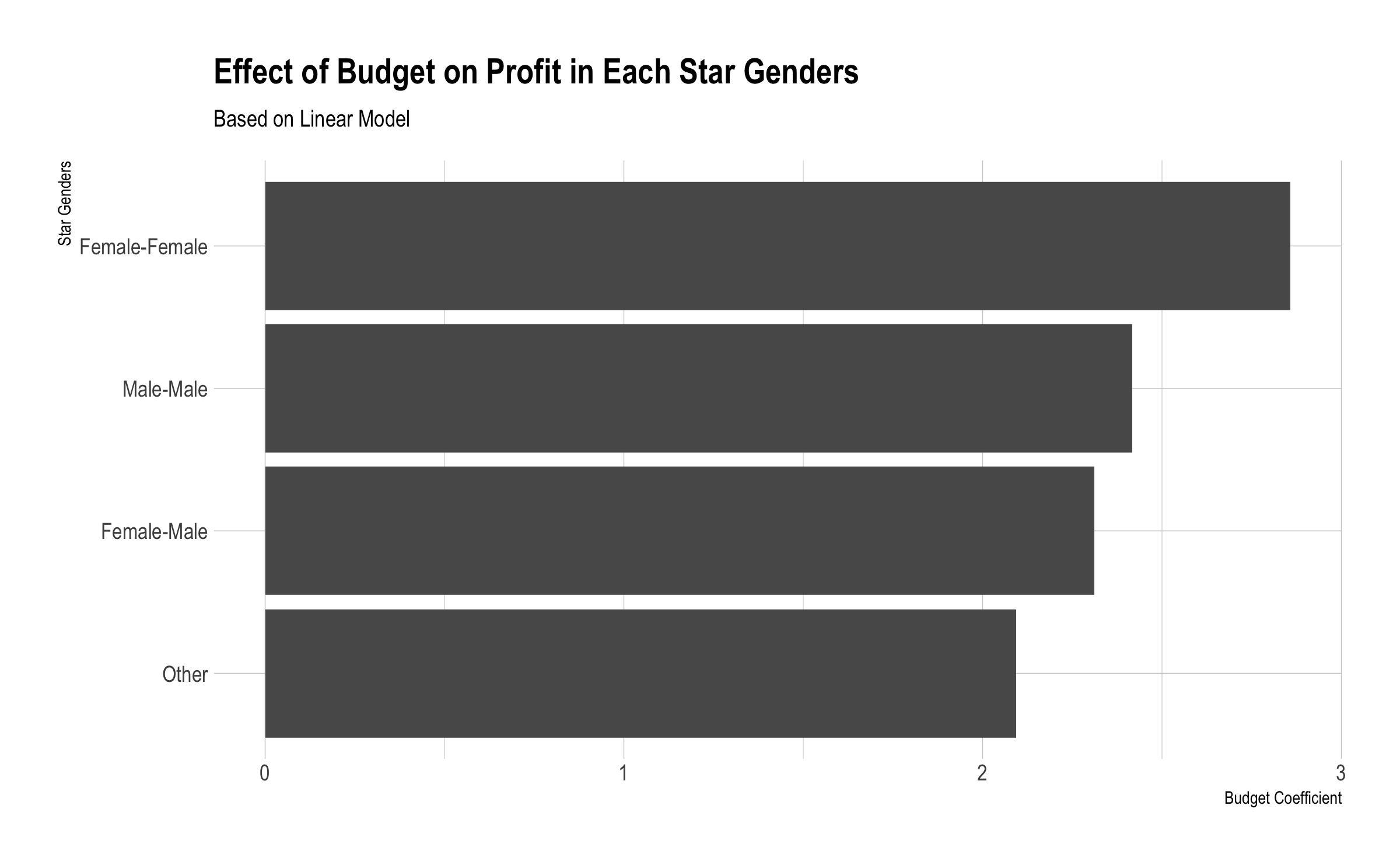
Does this prediction change based on the gender type of the main characters?
Similary, to identify the budget - profit relation for the star genders, linear modelling was applied in each star gender categories (male-female, female-female, female-male) seperately. The table below shows the coefficients of the budget in different star gender categories. The table below shows the budget coefficients on profit for each category.
Can we see differences in the effect regarding the movie production studio?
As majority of the studios have 2 or less movies in the given dataset, the linear model couldn’t be applied on those. In the table below, the budget coeffients and other statistics were shown for each studio. The test showed that, in the scope of most of the studios, the budget coefficient and relation significance vary a lot.
Does this prediction change based on the year?
As we did on the previous comparisons, to determine the changes on budget - profit relation over years, linear modelling was applied in each star years seperately. The table below shows the coefficients of the budget in different years. As the numbers of movies before 1975 was too low, those are omitted from analysis.
#> Warning: All elements of `...` must be named.
#> Did you want `data = c(movieId, title, genres, budget, profit, studio, star_female,
#>     star_male, star_unknown)`?
The graph shows that after the begining of 2000’s, the effect of bugget on the income started to increase slightly.