3 Numeric/ integer variables: Recoding to numeric, checking numeric variables and creating new variables by calculation

Data Wrangling Recipes in R: Hilary Watt.

This section for variables that are already numeric/ integer, or that you want to be numeric…

See chapter on factor variables to recode numeric data into categories such as into fifths or by clinical/ meaningful cut-offs…

Debugging AA: Support each other to debug & to factor debugging into your time-lines by joining Debugging Allowance Alliance. You need to form your own branch with your mates.

Firstly we show the data-type:

class(anaemia$hb_post) #show original data type

## [1] "integer"

is.numeric(anaemia$hb_post)

## [1] TRUE

is.integer(anaemia$hb_post)

## [1] TRUE

sum(is.na(anaemia$hb_post)) # count NAs

## [1] 15

anaemia$hb_post <- as.integer(anaemia$hb_post)   # does not change anything here - already integer which is appropriate
summary(anaemia$hb_post) # summary with min, max, mean, median for numeric/ integer data

##    Min. 1st Qu.  Median    Mean 3rd Qu.    Max.    NA's 
##   67.00   90.00   98.00   98.74  106.00  142.00      15

This chapter starts with variables which are already appropriately coded as integer or numeric. Then it teaches creation of new numeric variables. The final part covers converting to numeric, addressing issues such as stripping out units and similar.

3.1 Summarising variables and histograms: watching out for errors and assessing shape of distributions and what data is available

This is the next step once R recognises the relevant variables as numeric. Be alert to errors, by noticing impossible maximum and minimum values, which can be seen with summary() command or occasionally table() is more useful for integers with few values.

summary() summarises variables, with summary presented depending on R data-type.

For integer/numerical variables, summary() outputs the mean, median, range (min / max), intequartile range, and number of missing (NA) values. For categorical (factor) variables, summary() produces the frequency of each factor level, including NAs For string variables, it gives their (maximum) length. ?summary gives further details.

summary(anaemia$rbc) # summary for one variable at a time

##    Min. 1st Qu.  Median    Mean 3rd Qu.    Max.    NA's 
##   0.000   0.000   1.000   2.224   3.000  46.000       9

summary(anaemia[c("hb_pre", "hb_post", "weight", "rbc", "plts")]) #  gives summary for each selected var in turn

##      hb_pre         hb_post           weight            rbc        
##  Min.   : 77.0   Min.   : 67.00   Min.   : 38.00   Min.   : 0.000  
##  1st Qu.:121.0   1st Qu.: 90.00   1st Qu.: 70.00   1st Qu.: 0.000  
##  Median :135.0   Median : 98.00   Median : 80.00   Median : 1.000  
##  Mean   :131.8   Mean   : 98.74   Mean   : 83.21   Mean   : 2.224  
##  3rd Qu.:144.0   3rd Qu.:106.00   3rd Qu.: 92.00   3rd Qu.: 3.000  
##  Max.   :185.0   Max.   :142.00   Max.   :999.00   Max.   :46.000  
##  NA's   :11      NA's   :15       NA's   :11       NA's   :9       
##       plts       
##  Min.   : 0.000  
##  1st Qu.: 0.000  
##  Median : 0.000  
##  Mean   : 0.645  
##  3rd Qu.: 1.000  
##  Max.   :16.000  
##  NA's   :9

table(anaemia$plts, exclude =NULL)  # useful for integer variables that take very few values

## 
##    0    1    2    3    4    5    6    7   11   13   16 <NA> 
##  725  123  108   36   22    4    6    3    1    2    1    9

Look for outliers on the histogram. It is important to keep outliers in your dataset, unless you have clinical/ expert knowledge that they must necessarily be errors. It might occasionally be useful to see whether their exclusion substantially affects results, and report this fact (focusing on results that include them). Although for some huge datasets, outliers are removed that seem implausible; it is essential to report this is any write-up.

Assess shape of distributions (by histogram) – whether we might assume Normality in any analysis or whether highly skewed and not possible. (Note that regression analysis requires Normality of residuals – which might be Normal even when outcome variable is somewhat skewed). Predictor variables don’t need to be Normal, but highly skewed ones mean outliers may be very influential on the result, which may often be undesirable….

Occasionally, there may be inconsistent units – resulting histogram may show 2 peaks at VERY different values. Watch out for this……

Missing data is often coded as 9, 99 or 999, or perhaps -1, -2. Hence 999 looks like missing data code. Ideally, we should have a code book giving this information.

# Assess distributions and further assess what is plausible
hist(anaemia$weight)    # simple coding is fine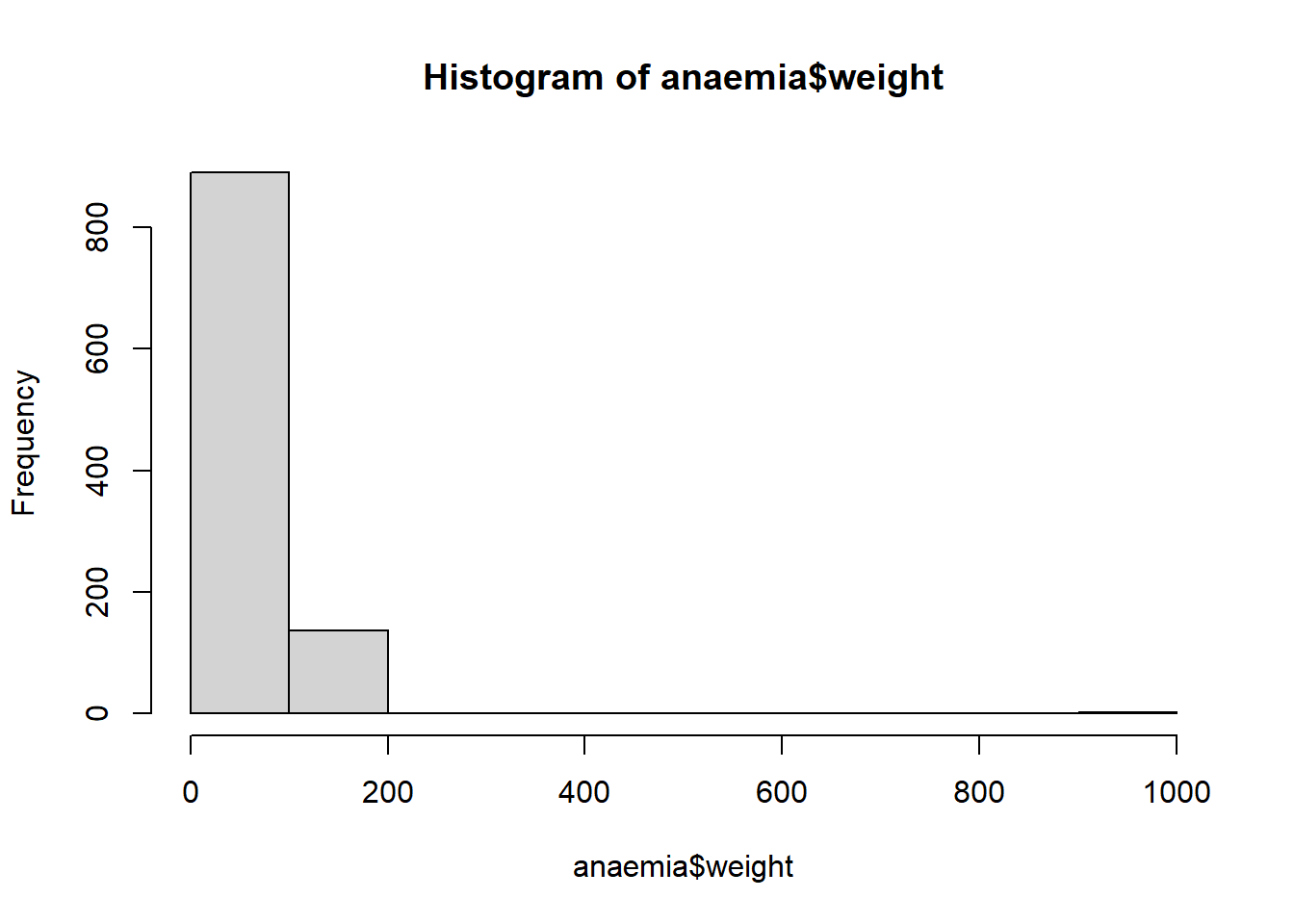

summary(anaemia$weight) # Show maximum is 999kg - impossible  

##    Min. 1st Qu.  Median    Mean 3rd Qu.    Max.    NA's 
##   38.00   70.00   80.00   83.21   92.00  999.00      11

There is no reason to make graphs fancier/ tidier, but it’s possible:

hist(anaemia$weight, main="Histogram of weight",
     xlab="weight (kg)", col="navy", border="white")
summary(anaemia$weight) # Show maximum is 999kg - impossible  

3.2 Recoding impossible values, usually to NA

# Set weight = NA where weight is 999
anaemia$weight[anaemia$weight == 999] <- NA

This evaluates whether or not: anaemia$weight == 999
double equals required to evaluate to see whether or not equal to

Then code followed only in that situation, which sets value to be NA (missing). This code would set all weight values to missing NA: anaemia$weight <- NA

Hence the one initial line above recodes this impossible value of weight=999 to missing. The following would also have worked here:

# set weight = NA where value is >900
anaemia$weight [anaemia$weight > 900] <- NA 
hist(anaemia$weight)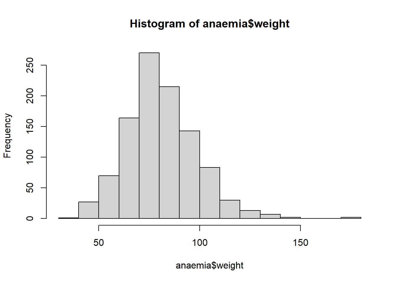

The above shows the revised histogram on valid weight values.

If we were able to check the correct value, we can use this to correct the value. This assumes we know their ID (id2 value), which is in quotes, because it is a string (non-numeric) variable:

# set weight = 78 where id2 is AB100
anaemia$weight [anaemia$id2 =="AB00000"] <- 78 

3.3 Sorting dataset to view data such as outliers

We might want to sort the data, so that we can look over the data more efficiently. This can allow easy inspection of patients with the lowest anaemia prior to operation (lowest hb_pre), where we can scroll through their values on all variables:

Using base R, with syntax df_name [row, column]. The following sorts the rows, and selects all columns, so there is a blank after the comma in column position:

anaemia <- anaemia[order(anaemia$hb_pre), ]

To look at each sex separately, since hb_pre is generally lower in females, sort firstly by sex and then by hb_pre within gender:

anaemia <- anaemia[order(anaemia$sex, anaemia$hb_pre), ]

By default, we sort lowest to highest. To reverse this order (highest to lowest), use the optional argument decreasing = TRUE.

anaemia <- anaemia[order(anaemia$hb_pre, decreasing = TRUE), ]

This is probably easier using Tidyverse’s arrange function

anaemia %>% arrange(hb_pre)   # order by hb_pre and print results

anaemia %>% arrange(sex, hb_pre)   # order by hb_pre within gender and print results

anaemia %>% arrange(sex, desc(hb_pre))   # order by sex then by hb_pre descending and print results

3.4 Creating new variables has 3 parts: create it, check it, save in tidy R script file

1. create the variable
2. check it (otherwise may analyse nonsense – ultimately saves time)
3. save commands that create/ modify/ check/ label variable into R script files (otherwise we lose our work).

Having a tidy R script file that reads in, cleans and modifies data is invaluable. Use if_else to amend by category and similar, which usefully retains the format & values of date & factor variables (hence is recommended over ifelse which is more problematic)).

Here are main operators, combine with brackets as necessary:

Operation	Description
+	addition
-	subtraction
*	multiplication
/	division
^	power

Commonly used mathematical functions are:

Operation	Description
log(xxx)	takes log to base e
log10(xxx)	takes log to base 10
exp(xxx)	takes the exponential
sqrt(xxx)	takes the square root

Calculating new variables

Creating new variables is done using the assignment operator <- as shown below. New variables are added to a dataframe by assigning a dataframe variable name (generally with 2 components of the variable name with a $, with data-frame name before $, so here anaemia$). For example, to create a variable calculating the change in haemoglobin from pre to post operation:

# create new variable called “hb_diff” for the change in
# haemoglobin pre and post operation.
anaemia$hb_diff <- anaemia$hb_post - anaemia$hb_pre
summary(anaemia$hb_diff) # summarise the new variable

##    Min. 1st Qu.  Median    Mean 3rd Qu.    Max.    NA's 
##  -80.00  -44.00  -34.00  -33.09  -24.00   33.00      17

summary(anaemia[c("hb_diff", "hb_pre", "hb_post")]) # check for NAs and for reasonable min, max, mean, SD

##     hb_diff           hb_pre         hb_post      
##  Min.   :-80.00   Min.   : 77.0   Min.   : 67.00  
##  1st Qu.:-44.00   1st Qu.:121.0   1st Qu.: 90.00  
##  Median :-34.00   Median :135.0   Median : 98.00  
##  Mean   :-33.09   Mean   :131.8   Mean   : 98.74  
##  3rd Qu.:-24.00   3rd Qu.:144.0   3rd Qu.:106.00  
##  Max.   : 33.00   Max.   :185.0   Max.   :142.00  
##  NA's   :17       NA's   :11      NA's   :15

View(anaemia[c("hb_diff", "hb_pre", "hb_post")]) # view relevant variables as visual check
View(anaemia[is.na(anaemia$hb_diff)==TRUE,  c("hb_diff", "hb_pre", "hb_post")]) # visual check when result in NA
anaemia[is.na(anaemia$hb_diff)==TRUE, c("hb_diff", "hb_pre", "hb_post")] # visual check when result in NA

If either hb_pre or hb_post are NA, then hb_diff will be NA (since it’s calculated from both of them). On this basis, the number of NAs for the hb_diff seems reasonable. We can substract mean of hb_pre from mean of hb_post to get (close to) mean of hb_diff (not precise agreement since each variable has a different number of NAs). We can visually inspect to check.

Example: finding body mass index, firstly checking weight and height are reasonable and recoding obvious errors/ missing data codes to NA. Then viewing result with summary and histogram.

summary(anaemia$height)

##    Min. 1st Qu.  Median    Mean 3rd Qu.    Max.    NA's 
##   1.360   1.650   1.730   1.761   1.800   9.000       9

anaemia$height [anaemia$height>2.5] <- NA
summary(anaemia$height)

##    Min. 1st Qu.  Median    Mean 3rd Qu.    Max.    NA's 
##   1.360   1.650   1.730   1.719   1.800   1.970      15

summary(anaemia$weight)

##    Min. 1st Qu.  Median    Mean 3rd Qu.    Max.    NA's 
##   38.00   70.00   80.00   81.42   92.00  174.00      13

anaemia$weight [anaemia$weight>800] <- NA
summary(anaemia$weight)

##    Min. 1st Qu.  Median    Mean 3rd Qu.    Max.    NA's 
##   38.00   70.00   80.00   81.42   92.00  174.00      13

anaemia$bmi <- anaemia$weight / (anaemia$height^2)
summary(anaemia$bmi) # 

##    Min. 1st Qu.  Median    Mean 3rd Qu.    Max.    NA's 
##   14.88   24.02   26.89   27.48   30.39   58.39      19

hist(anaemia$bmi)  # BMI (body mass index) is positively skewed as expected (not symmmetric, larger tail to right)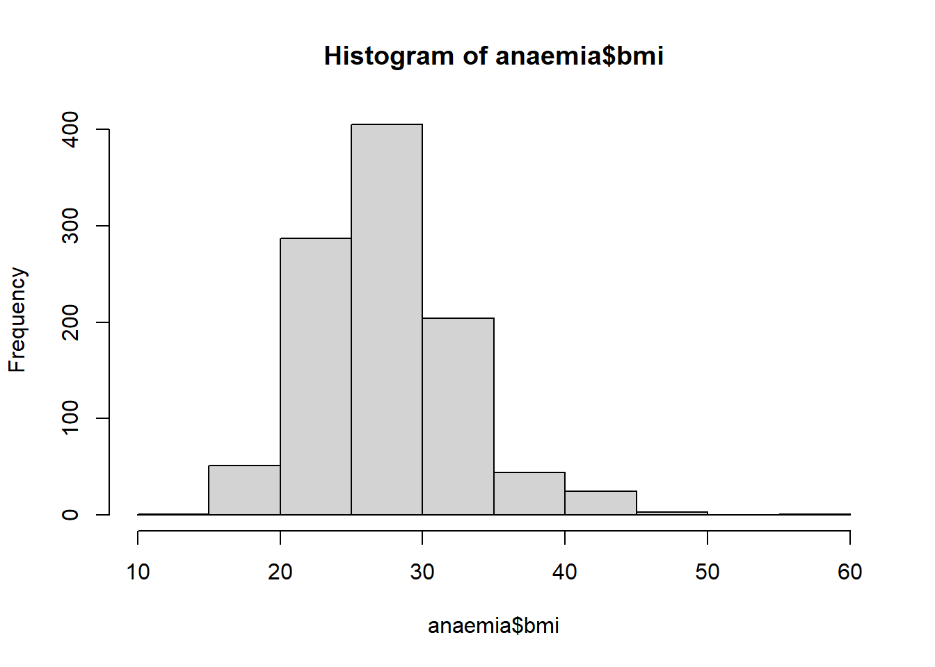

The above distribution looks reasonable for BMI.

3.5 Logs to calculate new variables, with attention on zeros, since log(0) =-Infinity

Remember to watch out of taking log of zero, since this evaluates to minus infinity. This destroys calculation of mean value and similar (mean is then also minus infinity in R). Recode these values to NA, or else recode zeros before taking logs. For instance, when people have zero nights stay in hospital post-operation, it is potentially reasonable to call that a stay of 0.5 days (rather than zero days). Then we can take readily take logs. We cannot take logs of negative values.

Finding log of the number of the duration of hospital stay post-operation. We often take logs of highly skewed variables, such as this, prior to analysis. Here we use log to base e (called the “natural log”).

Here we calculate the natural log of the duration of hospital stay post-operation.

# look at the help for the log function
?log

# generate a new variable called log_los_post by taking the log of los_post
anaemia$log_los_post <- log(anaemia$los_post)

# view the newly created variable alongside variable from which it was created.
# df[row.column] format used. Both the following work:
print(anaemia[c("los_post", "log_los_post")])

# print(anaemia[ , c("los_post", "log_los_post")]) # equivalent to above with extra comma

# check to see how many missing observations we have, compared to previous var
# log_post
summary(anaemia$log_los_post)

##    Min. 1st Qu.  Median    Mean 3rd Qu.    Max.    NA's 
##    -Inf   1.609   1.946    -Inf   2.398   5.247       9

# Recode -Inf to NA
anaemia$log_los_post[anaemia$log_los_post == -Inf] <- NA
summary(anaemia$log_los_post)  # Repeat summary command

##    Min. 1st Qu.  Median    Mean 3rd Qu.    Max.    NA's 
##   0.000   1.609   1.946   2.128   2.398   5.247      10

Note: \(\small{\log(0) = -\infty}\) which is minus infinity. This is considered different to \(\small{\log(\text{negative number})=}\)NaN (NaN = “not a number”, such as zero divided by zero)

Depending on context, it may be appropriate to take zeros to be a small value instead, to avoid ending up with minus infinity values after taking logs. Here it is not unreasonable to change to 0.5 days follow-up after operation, when currently it says zero (some people prefer to add 0.5 to all values). The following shows there are no minus infinity values and that the mean is reasonable, after this strategy.

# generate a new variable called log_los_post by taking the log of los_post
anaemia$los_post_0_5 <- anaemia$los_post   # copy to new variable
anaemia$los_post_0_5[anaemia$los_post_0_5==0] <- 0.5  # change zeros to 0.5 days in hospital
anaemia$log_los_post_0_5 <- log(anaemia$los_post_0_5) # works better for logs when reasonably justifiable
summary(anaemia$log_los_post_0_5)

##    Min. 1st Qu.  Median    Mean 3rd Qu.    Max.    NA's 
## -0.6931  1.6094  1.9459  2.1257  2.3979  5.2470       9

Other functions can be used similarly, but there is not necessarily a need to watch out of zeros or for negative values, according to the function.

3.6 Creating categorical variable from integer/ numeric

We might want to divide data into fifths, tenths or similar. We might want to divide into groups according to clinically meaningful cut-offs. See next chapter on factor variables for this.

3.7 Character to numeric/ integer data: changing how R recognises the data format, useful when data looks like numbers but not initially recognised as such

For any variables that look like numbers, but R calls them chr (character/ string) or factor variables, need to convert to number format, prior to analysis. If we convert to numeric, if some cells are not fully numeric, we may lose data. Check whether NAs are introduced in the process and whether they should appropriately contain data – see below.

as.numeric() converts to numeric format. The same issues/ code sequences apply to converting to integer using as.integer().

Firstly we show the data-type:

class(anaemia$hb_post) #show original data type

## [1] "integer"

is.numeric(anaemia$hb_post)

## [1] TRUE

is.integer(anaemia$hb_post)

## [1] TRUE

sum(is.na(anaemia$hb_post)) # count NAs

## [1] 15

anaemia$hb_post <- as.integer(anaemia$hb_post)   # does not change anything here - already integer which is appropriate
summary(anaemia$hb_post) # summary with min, max, mean, median for numeric/ integer data

##    Min. 1st Qu.  Median    Mean 3rd Qu.    Max.    NA's 
##   67.00   90.00   98.00   98.74  106.00  142.00      15

Example converting from character data to numeric, including checking that there are the same number of NAs or reasons for any extra ones

class(anaemia$height2) # gives data-type as recognised by R

## [1] "character"

str(anaemia$height2) # gives data-type and first few values

##  chr [1:1040] "1.71" "1.74" "1.67" "1.6799999" "1.8099999" "1.8" "1.75" ...

anaemia$height2.n <- as.numeric(anaemia$height2) # show NAs for new variable

## Warning: NAs introduced by coercion

subset(anaemia, select=c(height2.n, height2), subset=is.na(height2.n)==TRUE)  # shows NAs on new variable

The above shows that some cells with data resulted in NAs, even when there was data. The data concerned had units, which caused this issue. The following version correct this, removing the units “m” (but does not address the person with units “mm”)

str(anaemia$height2) # gives data-type and first few values

##  chr [1:1040] "1.71" "1.74" "1.67" "1.6799999" "1.8099999" "1.8" "1.75" ...

anaemia$height2.m <- as.numeric ( str_remove(anaemia$height2, "m") ) # remove units m (but not mm) - convert to numeric

## Warning: NAs introduced by coercion

subset(anaemia, select=c(height2.m, height2), subset=is.na(height2.m)==TRUE)  # shows NAs on new variable

summary(anaemia$height2.m)

##    Min. 1st Qu.  Median    Mean 3rd Qu.    Max.    NA's 
##   1.360   1.650   1.730   1.761   1.800   9.000      10

This version addresses the different units, including the need to change from mm to m for one person. This uses an ifelse statement. Note that the change in data-type to numeric needs to be within the ifelse statement, so that the division by 100 can be within this statement, since it applies only when initial units were mm.

anaemia$height2.mm <- ifelse (str_detect(anaemia$height2,"mm" ),
                              as.numeric( str_remove(anaemia$height2, "mm"))/100,
                              as.numeric (str_remove(anaemia$height2, "m"))) # convert from mm to m as required and removes unit 'm' in addition

## Warning in ifelse(str_detect(anaemia$height2, "mm"),
## as.numeric(str_remove(anaemia$height2, : NAs introduced by coercion

## Warning in ifelse(str_detect(anaemia$height2, "mm"),
## as.numeric(str_remove(anaemia$height2, : NAs introduced by coercion

subset(anaemia, select=c(height2.mm, height2), subset=is.na(height2.mm)==TRUE)  # shows NAs on new variable

summary(anaemia$height2.mm) # summarise new variable

##    Min. 1st Qu.  Median    Mean 3rd Qu.    Max.    NA's 
##   1.360   1.650   1.730   1.761   1.800   9.000       9

anaemia$height2.m <- NULL   # remove above version of data which isn't useful

Removing commas from numbers, so that they can be recognised as numbers:

str(anaemia$factorx)  ## see data-type and first few values

##  chr [1:1040] "59,228" "83,726" "972" "22,300" "46,033" "90,500" "87,079" ...

anaemia$factorx.n <- as.numeric ( str_remove(anaemia$factorx, ",") ) # remove commas - convert to numeric

## Warning: NAs introduced by coercion

anaemia[ is.na(anaemia$factorx.n)==TRUE, c("factorx.n", "factorx")]  # inspect NAs on new variable

summary(anaemia$factorx.n)  # see data

##    Min. 1st Qu.  Median    Mean 3rd Qu.    Max.    NA's 
##      96   24866   50451   50020   74850   99988      10

anaemia$factorx.n[anaemia$factorx=="higher than measurable by assay" ] <- 100000 # amend high value to plausible guess
summary(anaemia$factorx.n) # NAs reduced by one

##    Min. 1st Qu.  Median    Mean 3rd Qu.    Max.    NA's 
##      96   24869   50528   50068   74882  100000       9

There is one comment that there is a measure higher than assay can measure. This is was initially treated as missing, yet we have a lot of information about its value. It is better to treat it is a high value - perhaps taking the maximum value that the assay can measure. Or if that is not known, the highest value in the dataset, as in the script above.

Stripping out units kg from wgt variable: it is easier to convert into lower case first, so that we do not need to remove different versions of the units with lower case and upper case separately.

class(anaemia$wgt)

## [1] "character"

anaemia$wgt2.n <- str_to_lower(anaemia$wgt) # convert to lower case (units were kg, KG, Kg, g)
anaemia$wgt2.n <- str_remove(anaemia$wgt2.n, "kg" ) # now remove units from string
anaemia$wgt2.n <- as.numeric(anaemia$wgt2.n) # now can convert to numeric

## Warning: NAs introduced by coercion

summary(anaemia$wgt2.n) # shows mean etc since now numeric

##    Min. 1st Qu.  Median    Mean 3rd Qu.    Max.    NA's 
##   38.00   70.00   80.00   83.26   92.00  999.00      16

The check for missing data reveals 2 are missing, when they should not be:

If necessary, use an additional str_remove() command:

anaemia$wgt2 <- str_remove(str_remove(anaemia$wgt, “kg”), “KG”)

Here, there is an alternative, with a call to ignore the case:

anaemia$wgt2 <- str_remove(anaemia$wgt, regex("KG", ignore_case=TRUE)

More flexible string commands, for removing characters: https://evoldyn.gitlab.io/evomics-2018/ref-sheets/R_strings.pdf

See character variable section for detailed information on dividing strings into 2 component parts. However, the above covers the main issues

3.8 Recoding (ordered) factor variable into numeric/ integer

Hilary Watt

Usually, factor variables have named categories. We can convert these into numbers, where the first category becomes 1, the second becomes 2 and so on – table() shows the order. There is the option to re-order categories first, to give different numbers as desired (see 4.3). To convert var1_factor to var1_integer, with dataframe named df:

df$var1_integer <- as.integer (df$var1_factor)

WARNING: Sometimes we see numbers for each level of the factor variable (which are category “names”). When converting to numbers using as.numeric() or as.integer() will change these to numerical values 1,2,3, 4, 5,…. (rather than numbers that you see).

Confusing example converting from factor variable (assumes first step done earlier), where numbers do not end up as values initially shown. Numbers relate to numbering the different levels as level 1, 2, 3, 4,…

anaemia$plts.f <- as.factor(anaemia$plts) # for variables that are initially factor but look numeric
class(anaemia$plts.f) # find variable type

## [1] "factor"

anaemia$plts2 <- as.numeric(anaemia$plts.f) # convert to number
table(anaemia$plts.f, anaemia$plts2)  # shows disagreement between factor 'number' and numeric value

##     
##        1   2   3   4   5   6   7   8   9  10  11
##   0  725   0   0   0   0   0   0   0   0   0   0
##   1    0 123   0   0   0   0   0   0   0   0   0
##   2    0   0 108   0   0   0   0   0   0   0   0
##   3    0   0   0  36   0   0   0   0   0   0   0
##   4    0   0   0   0  22   0   0   0   0   0   0
##   5    0   0   0   0   0   4   0   0   0   0   0
##   6    0   0   0   0   0   0   6   0   0   0   0
##   7    0   0   0   0   0   0   0   3   0   0   0
##   11   0   0   0   0   0   0   0   0   1   0   0
##   13   0   0   0   0   0   0   0   0   0   2   0
##   16   0   0   0   0   0   0   0   0   0   0   1

If we want the number that appears for each category become its numeric value, we need to use as.numeric(as.character()), so that the numbers we see is what we get. May often be appropriate to use: as.integer(as.character()). Note: if any factor level has coded that is not fully numeric, this will result in NA.

anaemia$plts.f.n <- as.numeric(as.character(anaemia$plts.f))
table(anaemia$plts.f.n, anaemia$plts.f)

##     
##        0   1   2   3   4   5   6   7  11  13  16
##   0  725   0   0   0   0   0   0   0   0   0   0
##   1    0 123   0   0   0   0   0   0   0   0   0
##   2    0   0 108   0   0   0   0   0   0   0   0
##   3    0   0   0  36   0   0   0   0   0   0   0
##   4    0   0   0   0  22   0   0   0   0   0   0
##   5    0   0   0   0   0   4   0   0   0   0   0
##   6    0   0   0   0   0   0   6   0   0   0   0
##   7    0   0   0   0   0   0   0   3   0   0   0
##   11   0   0   0   0   0   0   0   0   1   0   0
##   13   0   0   0   0   0   0   0   0   0   2   0
##   16   0   0   0   0   0   0   0   0   0   0   1

Converting an (ordered) factor to numerical values is easier, when the orders are in some appropriate logical order, and we’ve happy for them to be numbered 1, 2, 3,… in sequence. Firstly, check what order the elements appear in. If this is not satisfactory, then reorder as follows:

table(anaemia$operat) #checking order

## 
##            Elective Emergency   Salvage    Urgent 
##         9       710        56         2       263

anaemia$operat.f <- factor(anaemia$operat, levels=c("Elective", "Urgent", "Emergency", "Salvage")) # change order
table(anaemia$operat.f)  # table shows new order

## 
##  Elective    Urgent Emergency   Salvage 
##       710       263        56         2

anaemia$operat.n <- as.integer(anaemia$operat.f) # convert to integer
table(anaemia$operat.n)  # shows values 1, 2, 3, 4

## 
##   1   2   3   4 
## 710 263  56   2

This is ordered from least urgent to most urgent. Although salvage might not necessarily fit in here. Perhaps it is more appropriate that such operations are excluded from the categorisation by urgency. We can specify only the other 3 categories to achieve this as follows:

table(anaemia$operat) #checking order

## 
##            Elective Emergency   Salvage    Urgent 
##         9       710        56         2       263

anaemia$operat.f2 <- factor(anaemia$operat, levels=c("Elective", "Urgent", "Emergency")) # change order & specify only relevant categories  since salvage does not necessarily fit into this ordering
table(anaemia$operat.f2)  # table shows new order

## 
##  Elective    Urgent Emergency 
##       710       263        56

anaemia$operat.n2 <- as.integer(anaemia$operat.f2) # convert to integer
table(anaemia$operat.n2)  # shows values 1, 2, 3

## 
##   1   2   3 
## 710 263  56

In practice, R treats uses the number associated with the factor level in some analyses (numbers 1, 2, 3, 4… for each category), even when we do not directly convert to numbers in this manner. However, converting to numeric format means that the variable is routinely treated as numeric in analyses.

3.9 Logicals to numeric, which are useful for indicator variables: TRUE becomes 1, FALSE becomes 0.

This illustrates firstly creating a logical TRUE/ FALSE variable, here indicating urgent (derived from operat variable). Then creating such a variable, whilst simultaneously converting to integer type. Note this is in line with the convention to code Yes=1 and No=0, which is very useful.

anaemia$urgent <- anaemia$operat=="Urgent"   # create logical from operat variable to denote urgent operation
table(anaemia$urgent)  # show variable

## 
## FALSE  TRUE 
##   777   263

anaemia$urgent <- as.integer( anaemia$operat=="Urgent")
table(anaemia$urgent)  # shows values 1, 2, 3

## 
##   0   1 
## 777 263

See character variable section for detailed information tidying up string variables (which includes doing this prior to converting to numeric). However, the above covers the main issues

---

The main dataset is called anaemia, available here: https://github.com/hcwatt/data_wrangling_open.

Data Wrangling Recipes in R: Hilary Watt. PCPH, Imperial College London.