Differential abundance analysis at guide level
There is classic edgeR and glm edgeR.
## Create the design matrix{-}
For further statistical modeling using edgeR, we now need to define a design matrix.
          (Intercept) groupToxA groupToxB
Control_2           1         0         0
Control_1           1         0         0
ToxA_2              1         1         0
ToxA_1              1         1         0
ToxB_2              1         0         1
ToxB_1              1         0         1
attr(,"assign")
[1] 0 1 1
attr(,"contrasts")
attr(,"contrasts")$group
[1] "contr.treatment"
0.2 Classic edgeR
0.2.1 Fit a model when there is no biological replicates
While it’s generally advisable to include biological replicates in experimental designs for statistical rigor and robust conclusions, there may be situations in CRISPR screens where researchers choose not to include them initially, especially in exploratory phases. The decision often involves a trade-off between the depth of analysis and the available resources. However, as the study progresses and findings are prioritized, additional experiments with biological replicates are often conducted to validate and strengthen the results. In instances where biological replicates are unavailable, they are not ideal but classic edgeR provides two alternative solutions: one involves the exactTest, and the other employs the Generalized Linear Model Likelihood Ratio Test (glmLRT). In such scenarios, a crucial step is to determine a sensible estimate for common Biological Coefficient of Variation (BCV). However, the p-values and the number differentially abundant guides will depend on the bcv. Subsequently, this estimate is utilized as follows:
bcv <- 0.6
yy.norm.no_biorep <- DGEList(counts = yy.norm$counts[, c(2, 4, 6)],
    samples = yy.norm$samples[c(2, 4, 6), ], genes = yy.norm$genes)
et <- exactTest(yy.norm.no_biorep, dispersion = bcv^2, pair = c(1,
    3))
head(topTags(et, n = Inf))
Comparison of groups: ToxB-Control
Symbol UID seq
HGLibA_56745 ZNF784 HGLibA_56745 GCAAGCTGTAGTGCGCGCGC
HGLibA_62457 hsa-mir-590 HGLibA_62457 TTATTCATAAAAGTGCAGTA
HGLibA_04839 BRPF1 HGLibA_04839 TACTGCTGTGGCCCACGCCG
HGLibA_39135 PSMC3IP HGLibA_39135 AATCGTGGCCCTCACTGCTA
HGLibA_39953 RAB44 HGLibA_39953 CAAGATGACCAGCCGCCTGC
HGLibB_51676 TRPC5 HGLibB_51676 CTCCCGACTGAACATCTATA
logFC logCPM PValue FDR
HGLibA_56745 16.40706 13.54169 4.396582e-10 2.458876e-05
HGLibA_62457 15.52052 12.65606 2.421539e-09 6.771472e-05
HGLibA_04839 14.37376 11.51312 2.197430e-08 2.349355e-04
HGLibA_39135 14.36467 11.51097 2.237347e-08 2.349355e-04
HGLibA_39953 14.35794 11.49787 2.266119e-08 2.349355e-04
HGLibB_51676 11.58312 12.08571 2.749944e-08 2.349355e-04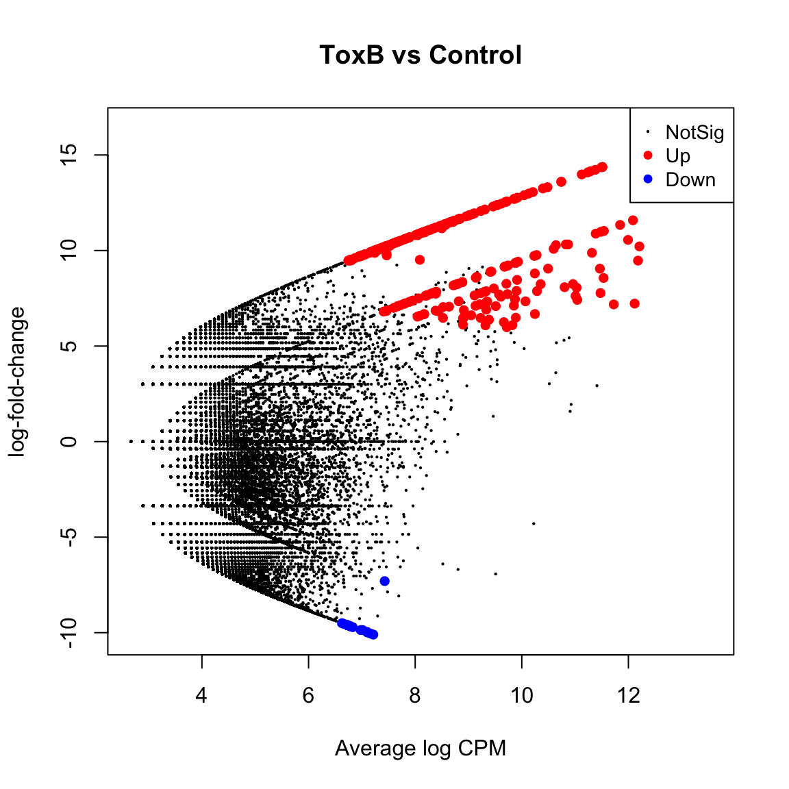
fit <- glmFit(yy.norm.no_biorep, dispersion = bcv^2)
lrt <- glmLRT(fit, coef = "y$samples$groupToxA")
topTags(lrt)
Coefficient: y$samples$groupToxA
Symbol UID seq logFC
HGLibB_38324 PRDM13 HGLibB_38324 GCAAGTACCTGTCAGACCGC 13.79029
HGLibB_04039 B4GALT7 HGLibB_04039 GCGAGGACGACGAGTTCTAC 13.55125
HGLibA_20923 HBEGF HGLibA_20923 GCCCTCTCCGAAGCCGCTCC 13.38190
HGLibB_44908 SLC35B2 HGLibB_44908 TCCGCCTGAAGTACTGCACC 10.90573
HGLibB_42762 SBSPON HGLibB_42762 GACAAGCTACGTCTCCACAC 12.68573
HGLibB_20894 HBEGF HGLibB_20894 TCTTGAACTAGCTGCCACCC 10.36379
HGLibB_23505 IQGAP3 HGLibB_23505 CACTCACAGGCTGCCCAGCC 12.37695
HGLibA_07161 CAPN15 HGLibA_07161 CATGTCGTCCACCAGCACCG 12.08184
HGLibA_56457 ZNF649 HGLibA_56457 ACTTAAGCTGTGACTTGCTG 11.97552
HGLibA_55349 ZKSCAN2 HGLibA_55349 ACCAGTGAAAGATGTCCACG 11.95656
logCPM LR PValue FDR
HGLibB_38324 10.887298 32.72439 1.061960e-08 0.0004436210
HGLibB_04039 10.649647 31.80684 1.702923e-08 0.0004436210
HGLibA_20923 10.640050 31.15712 2.379643e-08 0.0004436210
HGLibB_44908 11.410148 30.37388 3.562930e-08 0.0004981600
HGLibB_42762 9.912502 28.48975 9.419562e-08 0.0009711574
HGLibB_20894 11.041123 28.29456 1.041884e-07 0.0009711574
HGLibB_23505 9.517303 27.30909 1.733939e-07 0.0013853431
HGLibA_07161 9.336969 26.18251 3.106240e-07 0.0020335084
HGLibA_56457 9.198546 25.77718 3.831925e-07 0.0020335084
HGLibA_55349 9.262887 25.70492 3.978110e-07 0.0020335084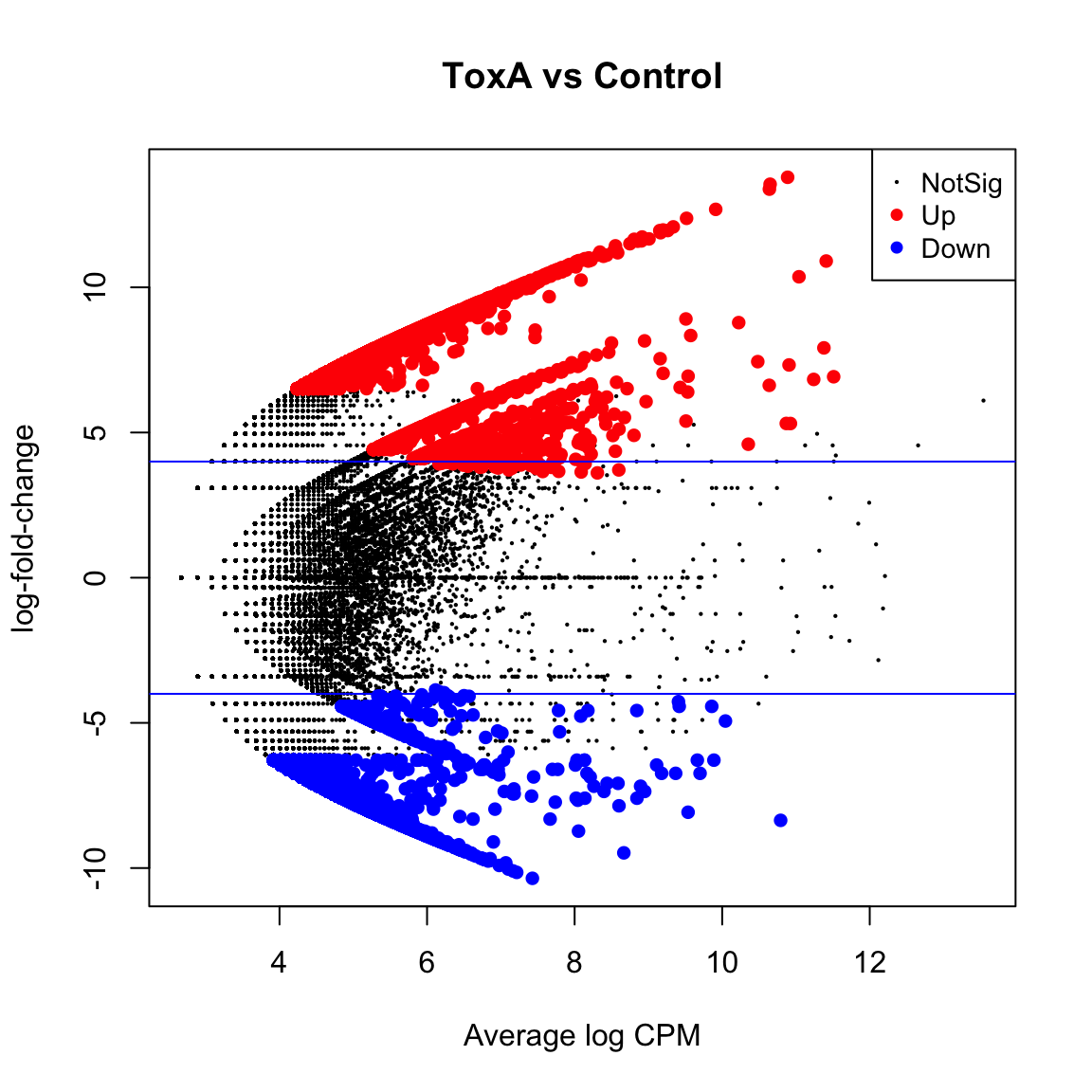
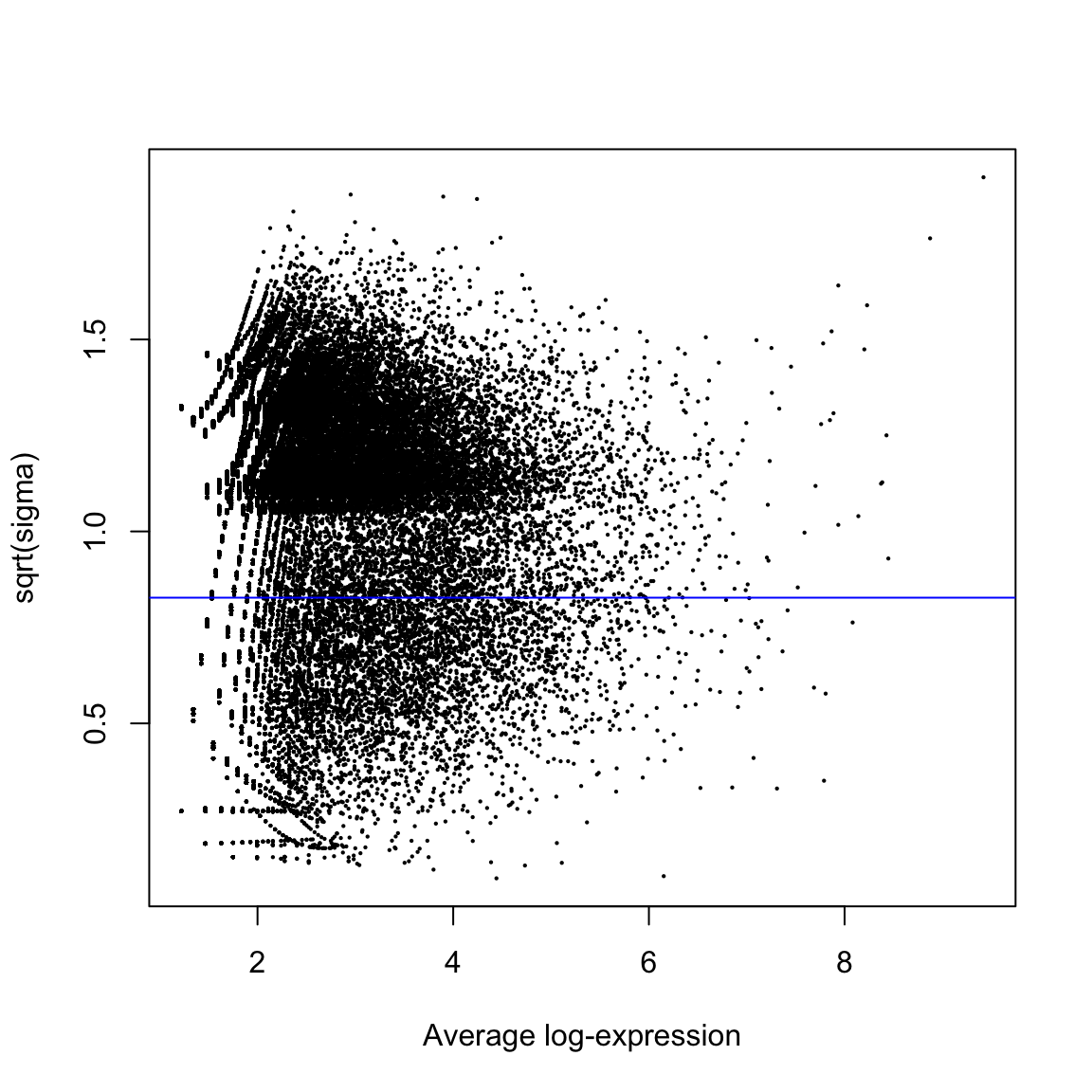
       (Intercept) groupToxA groupToxB
Down             0     22187     23861
NotSig        7965     27921     29501
Up 47962 5819 2565 (Intercept) groupToxA groupToxB
Down 0 6329 6416
NotSig 38603 47485 48871
Up 17324 2113 640toxa.vs.ctrl <- topTreat(tfit, coef = "groupToxA", n = Inf)
toxb.vs.ctrl <- topTreat(tfit, coef = "groupToxB", n = Inf)
head(toxa.vs.ctrl) Symbol UID seq logFC
HGLibA_32966 NUDT2 HGLibA_32966 ATGAGCACCAAGCCTACCGC 9.356170
HGLibA_36228 PGC HGLibA_36228 ACGACTCGCTGGGGTTGAAG 8.215204
HGLibA_38909 PRSS2 HGLibA_38909 CCACCCACTGTTCGCTGATG 8.625544
HGLibB_44452 SLC19A3 HGLibB_44452 CTGAATCACCAAGGCAATAA 8.319624
HGLibA_28771 MED20 HGLibA_28771 AACAGACATGATGCGGTCTA 7.952625
HGLibA_28209 MAP4 HGLibA_28209 CATACCGTAACTGTCTTTCA 8.233813
AveExpr t P.Value adj.P.Val
HGLibA_32966 5.682929 36.13809 4.663422e-07 0.00296124
HGLibA_36228 4.800247 33.54411 6.359671e-07 0.00296124
HGLibA_38909 4.665411 33.61408 6.369277e-07 0.00296124
HGLibB_44452 4.095367 33.24597 6.643360e-07 0.00296124
HGLibA_28771 3.444822 31.84156 8.013316e-07 0.00296124
HGLibA_28209 3.538396 31.62572 8.329187e-07 0.00296124[1] 55927 8[1] 8442 8 Symbol UID seq logFC
HGLibA_11002 CPSF3L HGLibA_11002 CTTTGGACACTTCGAGTGGC 9.248411
HGLibA_42364 RSU1 HGLibA_42364 TTCTTCAGTTCTGCGATGTT 9.248074
HGLibA_07730 CCDC22 HGLibA_07730 TCCAGAGCCACGGGAGTTCC 8.921697
HGLibA_52066 TTC19 HGLibA_52066 GTTCTGCGCAGCATAGATAC 8.853388
HGLibB_35573 PCLO HGLibB_35573 TGCTGAAGCGGATCCCTACC 8.282755
HGLibA_39824 RAB18 HGLibA_39824 GACATAGTAAACATGCTAGT 8.197197
AveExpr t P.Value adj.P.Val
HGLibA_11002 3.898377 40.11934 2.882188e-07 0.005210632
HGLibA_42364 3.898265 39.88013 2.962161e-07 0.005210632
HGLibA_07730 3.789472 38.23900 3.559404e-07 0.005210632
HGLibA_52066 3.766703 37.84200 3.726738e-07 0.005210632
HGLibB_35573 3.576501 34.45187 5.638743e-07 0.005877772
HGLibA_39824 3.547961 33.60296 6.305832e-07 0.005877772Biological variation
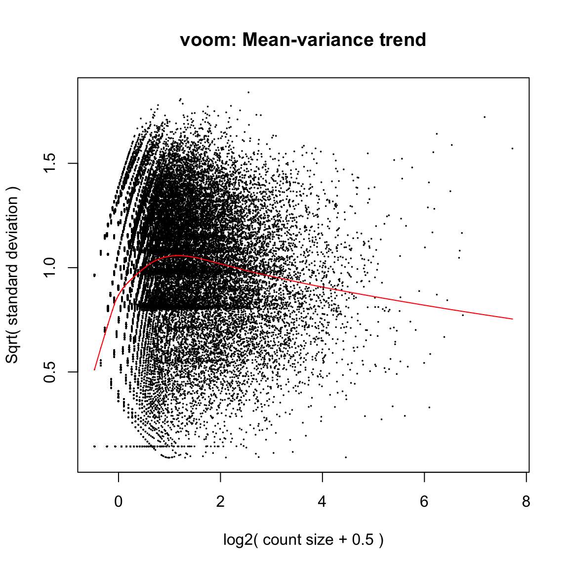
The vertical axis of the plot shows square-root dispersion, also known as biological coefficient of variation (BCV). For RNA-seq studies, the NB dispersions tend to be higher for genes with very low counts. The dispersion trend tends to decrease smoothly with abundance and to asymptotic to a constant value for genes with larger counts. From our past experience, the asymptotic value for the BCV tends to be in range from 0.05 to 0.2 for genetically identical mice or cell lines, whereas somewhat larger values (> 0.3) are observed for human subjects. The NB model can be extended with quasi-likelihood (QL) methods to account for gene-specific variability from both biological and technical sources7,12. Under the QL framework, the NB dispersion trend is used to describe the overall biological variability across all genes, and gene-specific variability above and below the overall level is picked up by the QL dispersion. In the QL approach, the individual (tagwise) NB dispersions are not used.
[1] 0.6331858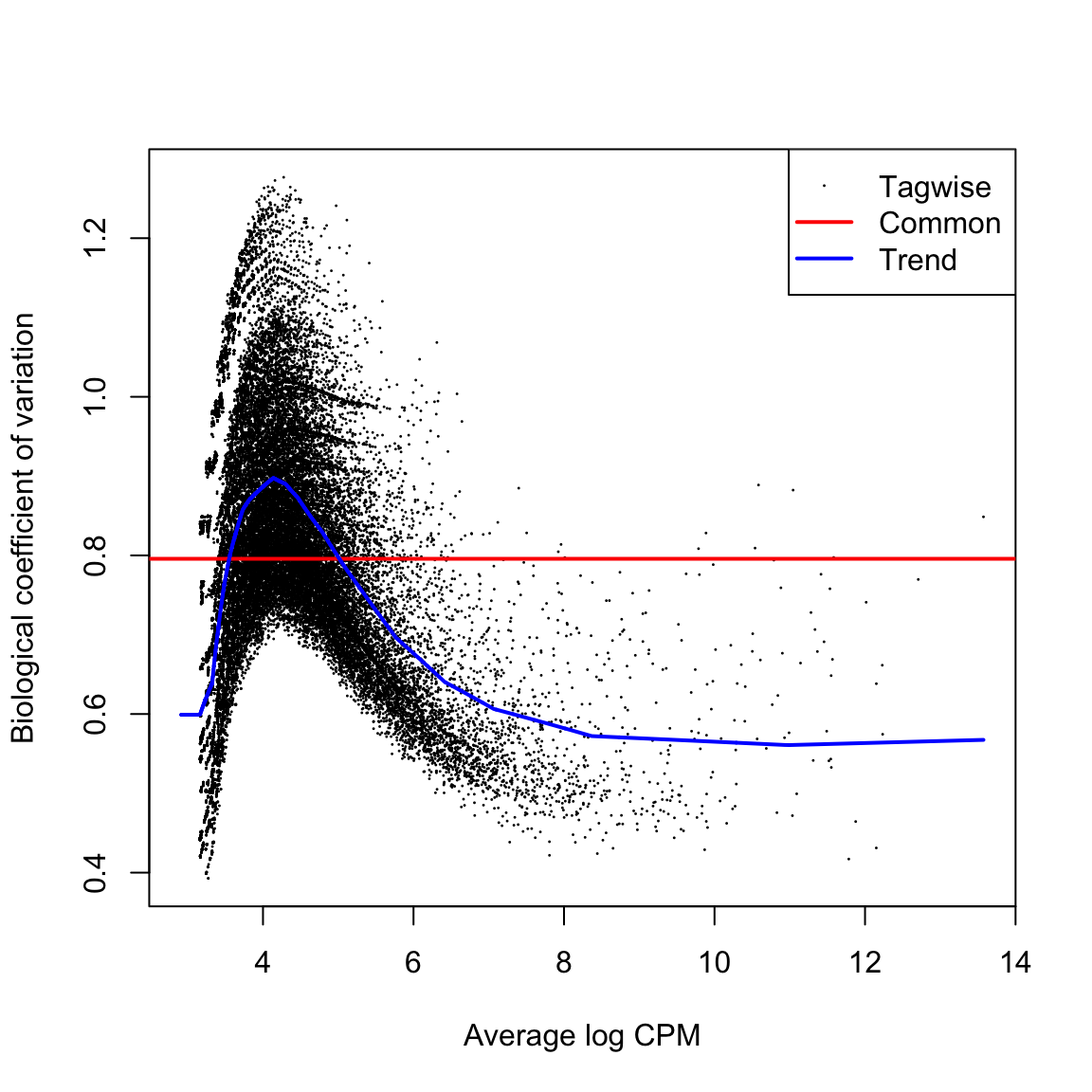 The square root of dispersion is the coefficient of biological variation (BCV). The common
BCV is on the high side, considering that this is a designed experiment using genetically
identical plants. The trended dispersion shows a decreasing trend with expression level. At
low logCPM, the dispersions are very large indeed.Note that only the trended dispersion is used under the quasi-likelihood (QL) pipeline. The tagwise and common estimates are shown here but will not be used further. The QL dispersions can be estimated using the glmQLFit function, and then be visualized with
the plotQLDisp function.
glmLRT edgeR
fit <- glmFit(yy.norm, design)
lrt <- glmLRT(fit, coef = "groupToxA")
topToxAvsCtrl.all <- topTags(lrt, n = Inf, sort.by = "PValue")$table
topToxAvsCtrl <- topTags(lrt, n = Inf, sort.by = "PValue")$table
dim(topToxAvsCtrl <- topToxAvsCtrl[topToxAvsCtrl$FDR < 0.05, ])
[1] 24709 8[1] 14953
topToxAvsCtrl$sgRNA <- rownames(topToxAvsCtrl)
topToxAvsCtrl$Gene_Regulation[topToxAvsCtrl$logFC >= 0] <- "Enriched in ToxA"
topToxAvsCtrl$Gene_Regulation[topToxAvsCtrl$logFC < 0] <- "Depleted in ToxA"
head(topToxAvsCtrl <- topToxAvsCtrl[topToxAvsCtrl$Symbol %in% alias2Symbol(topToxAvsCtrl$Symbol),
    ])
Symbol UID seq logFC
HGLibB_38324 PRDM13 HGLibB_38324 GCAAGTACCTGTCAGACCGC 11.209176
HGLibA_32966 NUDT2 HGLibA_32966 ATGAGCACCAAGCCTACCGC 11.594388
HGLibB_42762 SBSPON HGLibB_42762 GACAAGCTACGTCTCCACAC 12.255728
HGLibB_44908 SLC35B2 HGLibB_44908 TCCGCCTGAAGTACTGCACC 10.286574
HGLibB_45454 SLIT2 HGLibB_45454 TCTCTAGTTCTTTAAGATCC 11.404868
HGLibB_23505 IQGAP3 HGLibB_23505 CACTCACAGGCTGCCCAGCC 9.781491
logCPM LR PValue FDR
HGLibB_38324 10.829302 89.05910 3.831913e-21 2.143074e-16
HGLibA_32966 8.780164 73.01061 1.289546e-17 3.195504e-13
HGLibB_42762 9.530267 72.44893 1.714112e-17 3.195504e-13
HGLibB_44908 11.311403 69.70313 6.893661e-17 9.638544e-13
HGLibB_45454 8.763229 68.20288 1.475103e-16 1.649962e-12
HGLibB_23505 9.434533 66.97834 2.745064e-16 2.491273e-12
sgRNA Gene_Regulation
HGLibB_38324 HGLibB_38324 Enriched in ToxA
HGLibA_32966 HGLibA_32966 Enriched in ToxA
HGLibB_42762 HGLibB_42762 Enriched in ToxA
HGLibB_44908 HGLibB_44908 Enriched in ToxA
HGLibB_45454 HGLibB_45454 Enriched in ToxA
HGLibB_23505 HGLibB_23505 Enriched in ToxAglmQLFTest edgeR
   Min. 1st Qu.  Median    Mean 3rd Qu.    Max.
3.969 3.969 3.969 4.001 3.969 4.212 Coefficient: groupToxA
Symbol UID seq logFC
HGLibA_17021 FBXL8 HGLibA_17021 TCGCGGCCCGCGTCGAAGAG 7.921787
HGLibB_38324 PRDM13 HGLibB_38324 GCAAGTACCTGTCAGACCGC 11.208878
HGLibB_45542 SMAP1 HGLibB_45542 AAAGGATACTGATCTGTCTG 7.160555
HGLibA_08346 CD300LG HGLibA_08346 TCGAACCCGCTGATTTCCTC 7.108878
HGLibA_32966 NUDT2 HGLibA_32966 ATGAGCACCAAGCCTACCGC 11.594379
HGLibA_38909 PRSS2 HGLibA_38909 CCACCCACTGTTCGCTGATG 10.861509
HGLibA_38255 PQLC2 HGLibA_38255 GACATAATACACAGCCGTGT 6.337545
HGLibB_23505 IQGAP3 HGLibB_23505 CACTCACAGGCTGCCCAGCC 9.781238
HGLibB_44452 SLC19A3 HGLibB_44452 CTGAATCACCAAGGCAATAA 10.553844
HGLibB_44908 SLC35B2 HGLibB_44908 TCCGCCTGAAGTACTGCACC 10.286528
logCPM F PValue FDR
HGLibA_17021 8.707867 76.79967 4.247030e-05 0.1157827
HGLibB_38324 10.829302 79.73915 4.609961e-05 0.1157827
HGLibB_45542 7.743866 72.89386 5.051354e-05 0.1157827
HGLibA_08346 7.685687 72.60571 5.118125e-05 0.1157827
HGLibA_32966 8.780164 88.33076 6.707381e-05 0.1157827
HGLibA_38909 8.017500 82.15489 8.288510e-05 0.1157827
HGLibA_38255 7.819584 62.57073 8.354638e-05 0.1157827
HGLibB_23505 9.434533 65.83370 8.531276e-05 0.1157827
HGLibB_44452 7.706224 79.58075 9.093307e-05 0.1157827
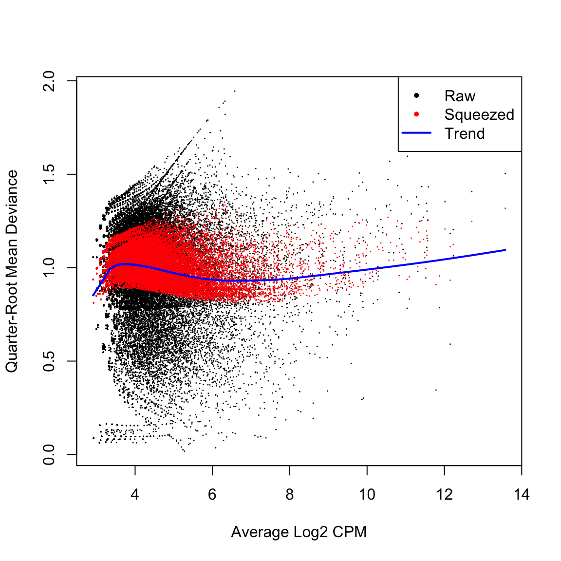
HGLibB_44908 11.311403 63.65797 9.494483e-05 0.1157827The large number of cases and the high variability means that the QL dispersions are not squeezed very heavily from the raw values. But here they are squeezed well. after BCV We then estimate the QL dispersions around the dispersion trend using glmQLFit.
Visualise hit guides
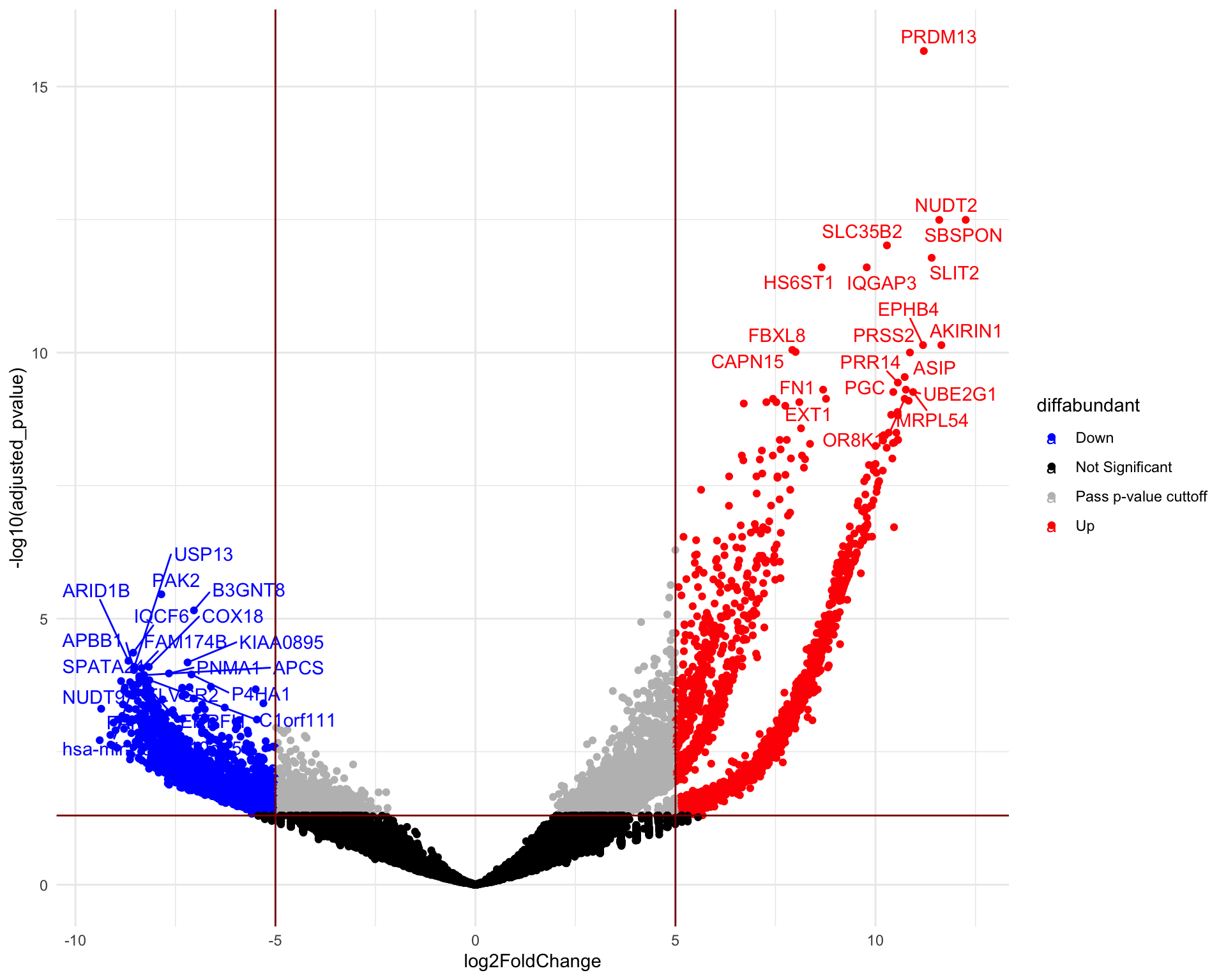
A volcano plot is a scatter plot that visualizes the differential abundance of guides. The fold change is typically displayed on the x-axis, while the y-axis represents the corresponding p-values. The significantly differentially abundant genes are the ones found in the upper-left and upper-right corners.
# remove rows that contain NA values
de <- topToxAvsCtrl.all[complete.cases(topToxAvsCtrl.all), ]
colnames(de)[colnames(de) == "logFC"] <- "log2FoldChange"
colnames(de)[colnames(de) == "PValue"] <- "pvalue"
colnames(de)[colnames(de) == "Symbol"] <- "gene_symbol"
colnames(de)[colnames(de) == "FDR"] <- "adjusted_pvalue"
de$diffabundant <- "Pass p-value cuttoff"
de$diffabundant[de$adjusted_pvalue > 0.05] <- "Not Significant"
de$diffabundant[de$log2FoldChange < -5 & de$log2FoldChange >= 5 & de$adjusted_pvalue <
    0.05] <- "Pass p-value & Log2FC cuttoff"
de$diffabundant[de$log2FoldChange >= 5 & de$adjusted_pvalue <= 0.05] <- "Up"
de$diffabundant[de$log2FoldChange < -5 & de$adjusted_pvalue <= 0.05] <- "Down"
head(de)
gene_symbol UID seq
HGLibB_38324 PRDM13 HGLibB_38324 GCAAGTACCTGTCAGACCGC
HGLibA_32966 NUDT2 HGLibA_32966 ATGAGCACCAAGCCTACCGC
HGLibB_42762 SBSPON HGLibB_42762 GACAAGCTACGTCTCCACAC
HGLibB_44908 SLC35B2 HGLibB_44908 TCCGCCTGAAGTACTGCACC
HGLibB_45454 SLIT2 HGLibB_45454 TCTCTAGTTCTTTAAGATCC
HGLibB_23505 IQGAP3 HGLibB_23505 CACTCACAGGCTGCCCAGCC
log2FoldChange logCPM LR pvalue
HGLibB_38324 11.209176 10.829302 89.05910 3.831913e-21
HGLibA_32966 11.594388 8.780164 73.01061 1.289546e-17
HGLibB_42762 12.255728 9.530267 72.44893 1.714112e-17
HGLibB_44908 10.286574 11.311403 69.70313 6.893661e-17
HGLibB_45454 11.404868 8.763229 68.20288 1.475103e-16
HGLibB_23505 9.781491 9.434533 66.97834 2.745064e-16
adjusted_pvalue diffabundant
HGLibB_38324 2.143074e-16 Up
HGLibA_32966 3.195504e-13 Up
HGLibB_42762 3.195504e-13 Up
HGLibB_44908 9.638544e-13 Up
HGLibB_45454 1.649962e-12 Up
HGLibB_23505 2.491273e-12 Up# Finally, we can organize the labels nicely using the 'ggrepel'
# package and the geom_text_repel() function
g_down <- which(de$log2FoldChange > 5 & de$adjusted_pvalue <= 0.05)
g_up <- which(de$log2FoldChange < -5 & de$adjusted_pvalue <= 0.05)
de$delabel <- NA
de$delabel[c(g_down[1:20], g_up[1:20])] <- de$gene_symbol[c(g_down[1:20],
g_up[1:20])]
# plot adding up all layers we have seen so far
ggplot(data = de, aes(x = log2FoldChange, y = -log10(adjusted_pvalue),
col = diffabundant, label = delabel)) + geom_point() + theme_minimal() +
geom_text_repel(max.overlaps = Inf) + scale_color_manual(values = c("blue",
"black", "gray", "red")) + geom_vline(xintercept = c(-5, 5), col = "darkred") +
geom_hline(yintercept = -log10(0.05), col = "darkred")