Differential abundance analysis at guide level
Differential abundance analysis in the context of CRISPR typically refers to the identification of significant differences in the abundance of sgRNAs between different experimental conditions or sample groups. Empirical analysis of Digital Gene Expression edgeR is one of the most widely used Bioconductor packages designed for the analysis of differential gene expression in RNA-seq data.
Here, we harness the robust capabilities of edgeR for differential expression analysis to precisely identify those sgRNAs that have a significant impact on the phenotype under investigation.
edgeR offers two distinct pipelines: the classic edgeR and the glm (generalized linear model) edgeR.
1. Classic edgeR: This pipelin is based on exactTest function and it can be used when there is no biological replicates in any condition.
2. edgeR glm (Generalized Linear Model): This pipeline splits into two distinct approaches with stricter error rate than classic edgeR:
a. edgeR glmLRT (Generalized Linear Model Likelihood Ratio Test): This approach relies on negative binomial generalized linear models, and the test employed is the Likelihood Ratio Test. This method ensures a more stringent control over the error rate compared to classic edgeR.
b. edgeR quasi glmQLFTest (Generalized Linear Model Quasi-Likelihood F-test): In this statistical methodology, negative binomial generalized linear models are employed, featuring F-tests instead of likelihood ratio tests. This pipeline is also controls the error rate better than classic edgeR, additionally edgeR-quasi excels in low-count situations.
Create the design matrix
For further statistical modeling using edgeR, we now need to define a design matrix containing the factors in the experiment.
(Intercept) groupToxA groupToxB
Control_2 1 0 0
Control_1 1 0 0
ToxA_2 1 1 0
ToxA_1 1 1 0
ToxB_2 1 0 1
ToxB_1 1 0 1
attr(,"assign")
[1] 0 1 1
attr(,"contrasts")
attr(,"contrasts")$group
[1] "contr.treatment"Fit a model when there is no biological replicates
While it’s generally advisable to include biological replicates in experimental designs for statistical rigor and robust conclusions, there may be situations in CRISPR screens where researchers choose not to include them initially, especially in exploratory phases. The decision often involves a trade-off between the depth of analysis and the available resources. However, as the study progresses and findings are prioritized, additional experiments with biological replicates are often conducted to validate and strengthen the results. In instances where biological replicates are unavailable, they are not ideal but classic edgeR provides two alternative solutions: one involves the exactTest, and the other employs the Generalized Linear Model Likelihood Ratio Test (glmLRT). In such scenarios, a crucial step is to determine a sensible estimate for common Biological Coefficient of Variation (BCV). However, the p-values will heavily depend on the initial BCV estimate. This BCV estimate is utilized and the statistical model is conducted as follows:
Classic edgeR
Here we subset only one biological replicate of each condition.
bcv <- 0.6
yy.norm.no_biorep <- DGEList(counts = yy.norm$counts[, c(2, 4, 6)], samples = yy.norm$samples[c(2,
4, 6), ], genes = yy.norm$genes)
et.toxb <- exactTest(yy.norm.no_biorep, dispersion = bcv^2, pair = c(1, 3))
et.toxa <- exactTest(yy.norm.no_biorep, dispersion = bcv^2, pair = c(1, 2))
head(topTags(et.toxb, n = Inf))Comparison of groups: ToxB-Control
Symbol UID seq logFC logCPM
HGLibA_56745 ZNF784 HGLibA_56745 GCAAGCTGTAGTGCGCGCGC 16.40706 13.54169
HGLibA_62457 hsa-mir-590 HGLibA_62457 TTATTCATAAAAGTGCAGTA 15.52052 12.65606
HGLibA_04839 BRPF1 HGLibA_04839 TACTGCTGTGGCCCACGCCG 14.37376 11.51312
HGLibA_39135 PSMC3IP HGLibA_39135 AATCGTGGCCCTCACTGCTA 14.36467 11.51097
HGLibA_39953 RAB44 HGLibA_39953 CAAGATGACCAGCCGCCTGC 14.35794 11.49787
HGLibB_51676 TRPC5 HGLibB_51676 CTCCCGACTGAACATCTATA 11.58312 12.08571
PValue FDR
HGLibA_56745 4.396582e-10 2.458876e-05
HGLibA_62457 2.421539e-09 6.771472e-05
HGLibA_04839 2.197430e-08 2.349355e-04
HGLibA_39135 2.237347e-08 2.349355e-04
HGLibA_39953 2.266119e-08 2.349355e-04
HGLibB_51676 2.749944e-08 2.349355e-04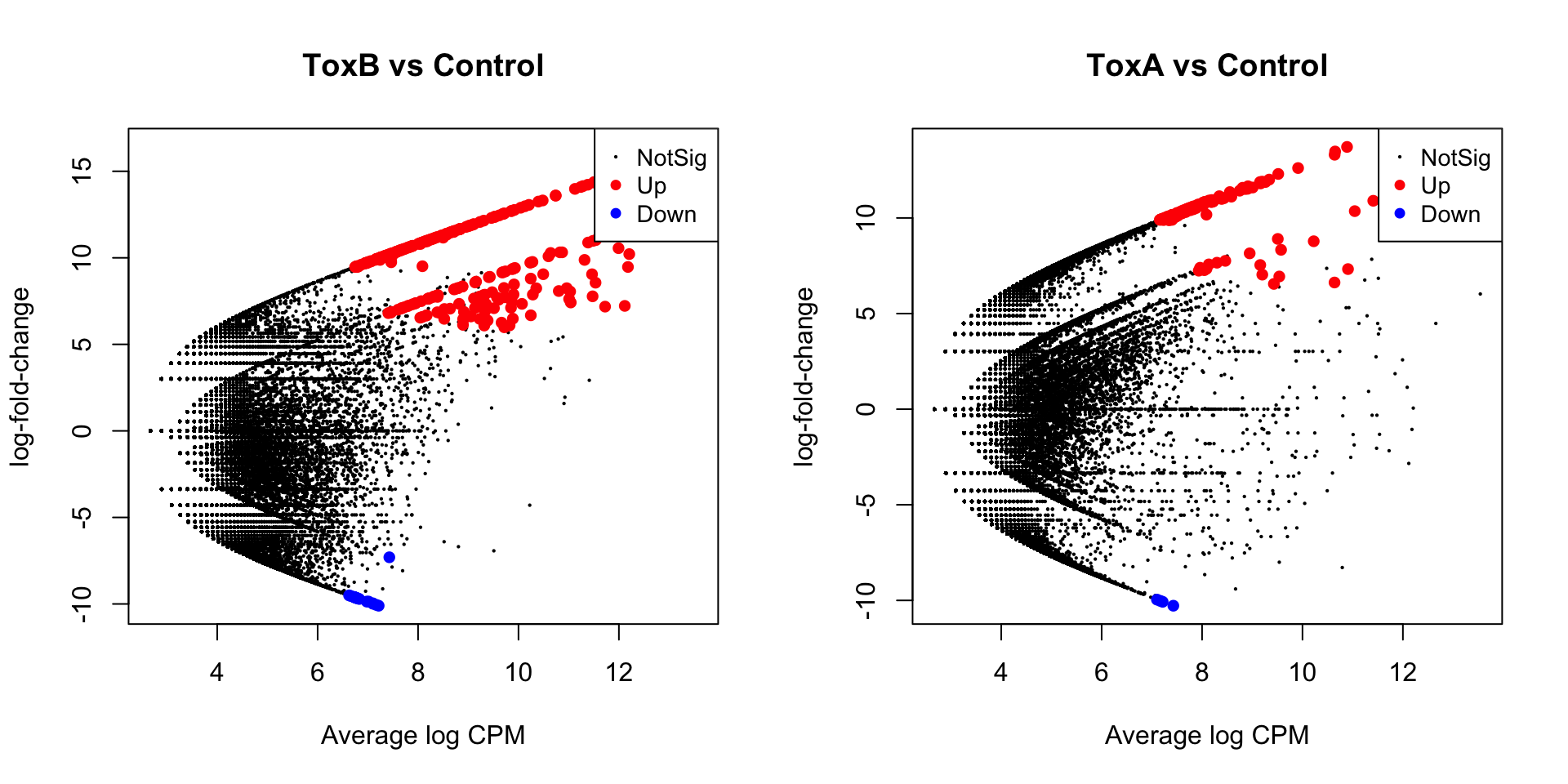
RStudioGD
2 write.csv(et.toxa, file = paste0("./tables/", Sys.Date(), "Classic_edgeR-ToxAvsCtrl-DE-sgRNAs.csv"))
edgeR glmLRT
par(mfrow = c(1, 2))
fit <- glmFit(yy.norm.no_biorep, dispersion = bcv^2)
lrt.toxa <- glmLRT(fit, coef = "y$samples$groupToxA")
lrt.toxb <- glmLRT(fit, coef = "y$samples$groupToxB")
topTags(lrt.toxa)Coefficient: y$samples$groupToxA
Symbol UID seq logFC logCPM
HGLibB_38324 PRDM13 HGLibB_38324 GCAAGTACCTGTCAGACCGC 13.79029 10.887298
HGLibB_04039 B4GALT7 HGLibB_04039 GCGAGGACGACGAGTTCTAC 13.55125 10.649647
HGLibA_20923 HBEGF HGLibA_20923 GCCCTCTCCGAAGCCGCTCC 13.38190 10.640050
HGLibB_44908 SLC35B2 HGLibB_44908 TCCGCCTGAAGTACTGCACC 10.90573 11.410148
HGLibB_42762 SBSPON HGLibB_42762 GACAAGCTACGTCTCCACAC 12.68573 9.912502
HGLibB_20894 HBEGF HGLibB_20894 TCTTGAACTAGCTGCCACCC 10.36379 11.041123
HGLibB_23505 IQGAP3 HGLibB_23505 CACTCACAGGCTGCCCAGCC 12.37695 9.517303
HGLibA_07161 CAPN15 HGLibA_07161 CATGTCGTCCACCAGCACCG 12.08184 9.336969
HGLibA_56457 ZNF649 HGLibA_56457 ACTTAAGCTGTGACTTGCTG 11.97552 9.198546
HGLibA_55349 ZKSCAN2 HGLibA_55349 ACCAGTGAAAGATGTCCACG 11.95656 9.262887
LR PValue FDR
HGLibB_38324 32.72439 1.061960e-08 0.0004436210
HGLibB_04039 31.80684 1.702923e-08 0.0004436210
HGLibA_20923 31.15712 2.379643e-08 0.0004436210
HGLibB_44908 30.37388 3.562930e-08 0.0004981600
HGLibB_42762 28.48975 9.419562e-08 0.0009711574
HGLibB_20894 28.29456 1.041884e-07 0.0009711574
HGLibB_23505 27.30909 1.733939e-07 0.0013853431
HGLibA_07161 26.18251 3.106240e-07 0.0020335084
HGLibA_56457 25.77718 3.831925e-07 0.0020335084
HGLibA_55349 25.70492 3.978110e-07 0.0020335084Coefficient: y$samples$groupToxB
Symbol UID seq logFC logCPM
HGLibA_56745 ZNF784 HGLibA_56745 GCAAGCTGTAGTGCGCGCGC 16.45477 13.54169
HGLibA_62457 hsa-mir-590 HGLibA_62457 TTATTCATAAAAGTGCAGTA 15.56822 12.65606
HGLibA_04839 BRPF1 HGLibA_04839 TACTGCTGTGGCCCACGCCG 14.42146 11.51312
HGLibA_39135 PSMC3IP HGLibA_39135 AATCGTGGCCCTCACTGCTA 14.41237 11.51097
HGLibA_39953 RAB44 HGLibA_39953 CAAGATGACCAGCCGCCTGC 14.40564 11.49787
HGLibB_00899 ADCK5 HGLibB_00899 CCTCGGAGCCCGCTATGTCA 14.27026 11.37898
HGLibA_03500 ATG5 HGLibA_03500 TTCCATGAGTTTCCGATTGA 14.19247 11.28652
HGLibA_25094 KLHDC10 HGLibA_25094 GTTTAAGGAATATGCTGTCC 14.13953 11.24048
HGLibB_43525 SERPINE1 HGLibB_43525 TCCACTGGCCGTTGAAGTAG 14.02994 11.12450
HGLibB_51676 TRPC5 HGLibB_51676 CTCCCGACTGAACATCTATA 11.58768 12.08571
LR PValue FDR
HGLibA_56745 42.97099 5.555765e-11 3.107173e-06
HGLibA_62457 39.55929 3.182494e-10 8.899368e-06
HGLibA_04839 35.14919 3.053877e-09 3.524250e-05
HGLibA_39135 35.11426 3.109157e-09 3.524250e-05
HGLibA_39953 35.08838 3.150759e-09 3.524250e-05
HGLibB_00899 34.56813 4.115905e-09 3.724658e-05
HGLibA_03500 34.26922 4.799120e-09 3.724658e-05
HGLibA_25094 34.06582 5.327885e-09 3.724658e-05
HGLibB_43525 33.64485 6.614986e-09 4.110626e-05
HGLibB_51676 32.99376 9.245512e-09 5.170737e-05plotMD(lrt.toxa, main = "ToxA vs Control")
abline(h = c(-3, 3), col = "blue")
plotMD(lrt.toxb, main = "ToxB vs Control")
abline(h = c(-3, 3), col = "blue")
RStudioGD
2 
lrt.toxb$table$Symbol <- lrt.toxb$genes$Symbol
write.csv(lrt.toxa$table, file = paste0("./tables/", Sys.Date(), "edgeR_glmLRT-ToxAvsCtrl-DE-sgRNAs.csv"))
write.csv(lrt.toxb$table, file = paste0("./tables/", Sys.Date(), "edgeR_glmLRT-ToxBvsCtrl-DE-sgRNAs.csv"))
datatable(format(lrt.toxa$table[order(lrt.toxb$table$PValue, decreasing = FALSE),
], format = "e", digits = 3))Fit a model when there are biological replicates
When there are a minimum of two biological replicates for each condition under consideration, the edgeR glm method performs better than classic edgeR in CRISPR experiments. To employ edgeR glm, it’s essential to estimate the dispersion parameter of the negative binomial (NB) distribution. This parameter is crucial as it accommodates the variability observed between biological replicates.
Dispersion estimates and biological variation
These estimates can be visualized with plotBCV function from edgeR.
[1] 0.6331858[1] 0.7957297 BCV is computed as the square root of common dispersion, which is 0.8 (larger than 0.3) in this experiment. This is high considering that genetically identical cells are used to deign the experiment. The trended dispersion shows that when the abundance gets higher, the variation decreases. At low logCPM, the dispersion is very large.
edgeR glmLRT
fit <- glmFit(yy.norm, design)
lrt <- glmLRT(fit, coef = "groupToxA")
lrt2.toxa <- topTags(lrt, n = Inf, sort.by = "PValue")$table
lrt <- glmLRT(fit, coef = "groupToxB")
lrt2.toxb <- topTags(lrt, n = Inf, sort.by = "PValue")$table
datatable(format(lrt2.toxa[order(lrt2.toxa$FDR, decreasing = FALSE), ], format = "e",
digits = 3))edgeR quasi
Both edgeR glm and edgeR quasi are viable options. So next we will continue analyzing the given example using edgeR quasi. It’s important to note that, under the quasi-likelihood (QL) pipeline, only the trended dispersion is utilized, not The tagwise and common estimates. The QL dispersions can be estimated by utilizing the glmQLFit function and subsequently visualized using the plotQLDisp function. Also note that the results of this pipeline can be quite conservative and as shown below, there mey be only a few or no significant hit can be detected.
Both edgeR glm and edgeR quasi are feasible choices. Therefore, we will proceed with the analysis of the provided example using edgeR quasi. It’s crucial to highlight that, within the quasi-likelihood (QL) pipeline, only the trended dispersion is employed, not the tagwise and common estimates. The QL dispersions can be estimated using the glmQLFit function and visualized through the plotQLDisp function. A graphical representation with plotQLDisp below depicts the quarter-root QL dispersion plotted against the average abundance of each gene. The estimates are presented for the raw dispersions (pre-empirical Bayes moderation), trended dispersions, and squeezed dispersions (post-empirical Bayes moderation). Additionally, it’s worth noting that the outcomes of this pipeline can be conservative, as demonstrated below, where only a few or no significant hits may be detected.

qlf.toxa <- glmQLFTest(fit, coef = "groupToxA")
qlf2.toxa <- topTags(qlf.toxa, n = Inf, sort.by = "PValue")$table
datatable(format(qlf2.toxa[order(qlf2.toxa$FDR, decreasing = FALSE), ], format = "e",
digits = 3))write.csv(qlf.toxa, file = paste0("./tables/", Sys.Date(), "-edgeR_glmQLF-with_biorep-ToxAvsCtrl-DE-sgRNAs.csv"))
qlf.toxb <- glmQLFTest(fit, coef = "groupToxB")
qlf2.toxb <- topTags(qlf.toxb, n = Inf, sort.by = "PValue")$table
datatable(format(qlf2.toxb[order(qlf2.toxb$FDR, decreasing = FALSE), ], format = "e",
digits = 3))