5 Modelling part

5.1 Prediction of the electricity consumption

Altough we already tried to figure out some patterns between characteristics of states and energy consumption, we will analyse the importance of the variables through a principal component analysis. It will allow us to know which variable are necessary to predict the energy consumption but also to confirm our previous analysis of the energy consumption.

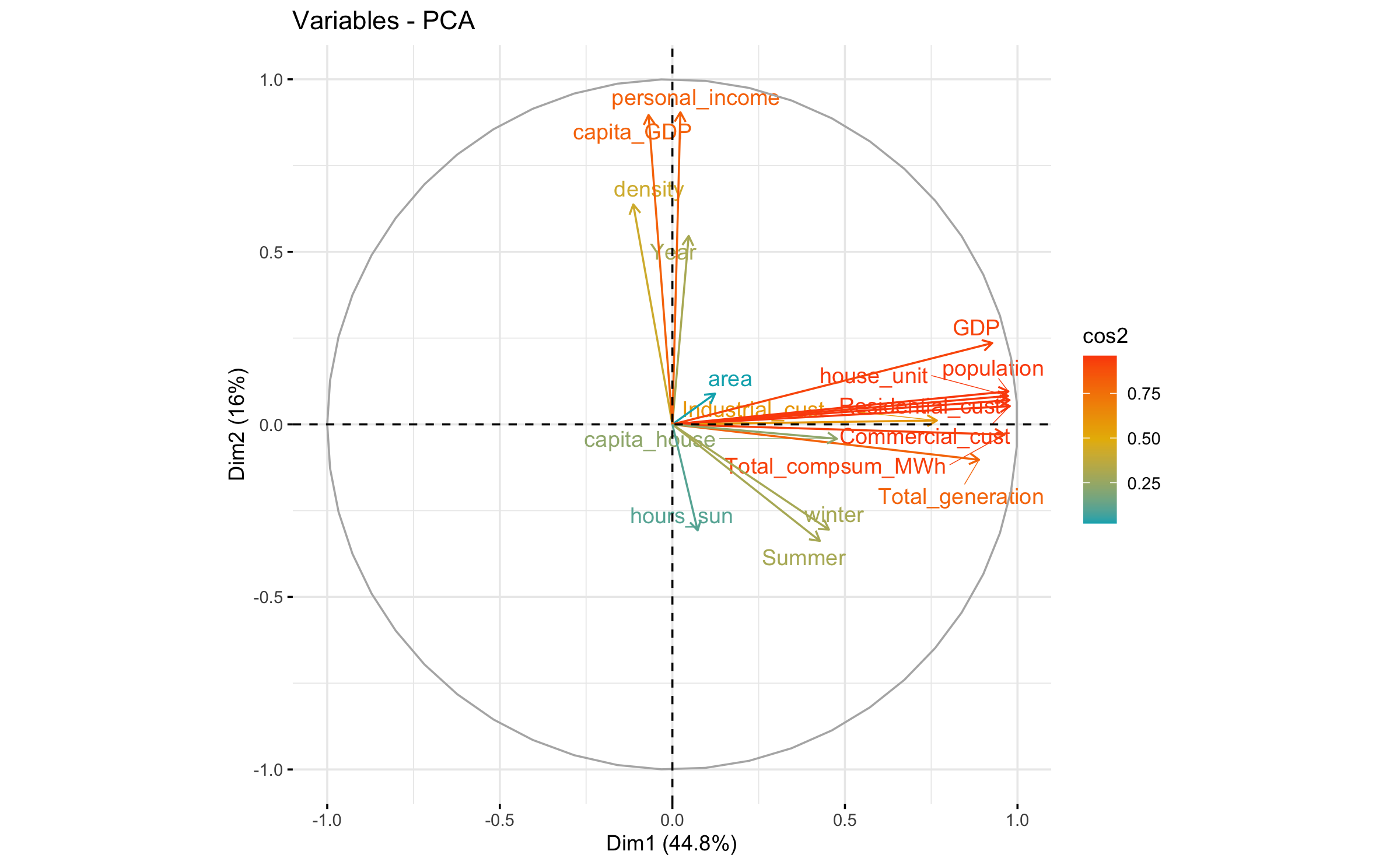
Figure 5.1: Principal component analysis

As we can see in the Principal Component Analysis (PCA) (Figure 5.1), there is two different groups playing different roles. It seems that energy consumption is not correlated to personal_income, capita_GDP, density and year. It totally confirms our previous analysis.

According to the Kaiser-Guttman rule, we should stop at Component 5. The Kaiser-Guttman rule states that components with an eigenvalue greater than 1 should be retained. We diplay this method in Figure 5.2.

Table 5.1: Eigenvalues of our variables

	eigenvalue	variance.percent	cumulative.variance.percent
Dim.1	7.623	44.842	44.8
Dim.2	2.728	16.049	60.9
Dim.3	1.996	11.742	72.6
Dim.4	1.224	7.201	79.8
Dim.5	1.080	6.351	86.2
Dim.6	0.744	4.378	90.6
Dim.7	0.569	3.344	93.9
Dim.8	0.401	2.358	96.3
Dim.9	0.237	1.395	97.7
Dim.10	0.158	0.927	98.6
Dim.11	0.143	0.841	99.4
Dim.12	0.040	0.237	99.7
Dim.13	0.027	0.160	99.8
Dim.14	0.016	0.093	99.9
Dim.15	0.011	0.063	100.0
Dim.16	0.002	0.013	100.0
Dim.17	0.001	0.004	100.0

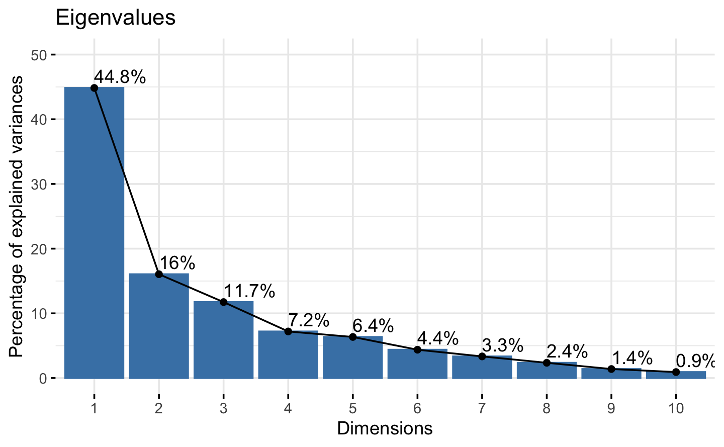
Figure 5.2: Kaiser-Guttman rule

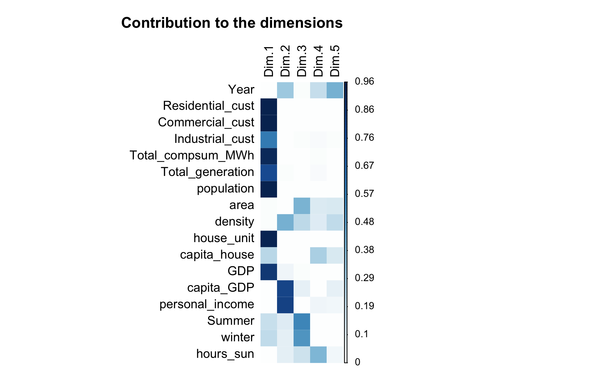
We will focus on the first dimension because the variable that we want to predict (Total_compsum_MWh) is in dimension one. We will also keep other variables that represent the most the principal dimension (Dim 1) because they are correlated to the variable “Total_compsum_MWh”.

The squared cosine shows the importance of a component for a given observation. The squared cosine indicates the contribution of a component to the squared distance of the observation to the origin (See Abdi and Williams 2010).

In our case, the variables contributing the most to the first component are the following:

• Residential_cust
• Commercial_cust
• Industrial_cust
• Total_compsum_MWh
• Total_generation
• population
• house_unit
• GDP

Below, we can see their contributions.

Table 5.2: Contribution of the variables

	Dim.1	Dim.2	Dim.3	Dim.4	Dim.5
Year	0.002	0.298	0.015	0.196	0.408
Residential_cust	0.954	0.005	0.007	0.008	0.001
Commercial_cust	0.956	0.003	0.006	0.008	0.001
Industrial_cust	0.587	0.000	0.011	0.026	0.018
Total_compsum_MWh	0.926	0.001	0.000	0.015	0.002
Total_generation	0.790	0.011	0.000	0.019	0.007
population	0.948	0.009	0.009	0.002	0.000
area	0.015	0.008	0.401	0.120	0.126
density	0.013	0.406	0.217	0.109	0.206
house_unit	0.946	0.007	0.008	0.009	0.001
capita_house	0.227	0.002	0.002	0.260	0.131
GDP	0.859	0.056	0.011	0.000	0.000
capita_GDP	0.005	0.804	0.081	0.003	0.082
personal_income	0.001	0.818	0.008	0.051	0.041
Summer	0.183	0.114	0.550	0.002	0.009
winter	0.206	0.093	0.499	0.006	0.000
hours_sun	0.005	0.094	0.171	0.389	0.047

Now, we can proceed to the modelling part.

First, we split the data into two parts:

• Training set
• Testing set

We chose to have a training set of 75% of the data and a testing set with the remaining ones.

5.1.1 Data splitting

set.seed(234)
index <- sample(x=c(1,2), size=nrow(jointurePCA), replace=TRUE, prob=c(0.75,0.25)) 
dat.tr <- jointurePCA[index==1,]
dat.te <- jointurePCA[index==2,]
# 1==training set, 2==test set

5.1.2 Model training

We build a multiple regression model to predict the consumption of energy. We will use all the principal variables that we selected in the PCA part.

Total_compsum_MWh~GDP + population + house_unit + Residential_cust + Commercial_cust + Industrial_cust + Total_generation

We used the AIC to select the best model possible. In the first attempt, GDP is removed.

Table 5.3: Total_compsum_MWh ~ population + house_unit + Residential_cust + Commercial_cust + Industrial_cust + Total_generation

Parameter	Estimate	Standard Error	P.value
(Intercept)	-1.59e+06	6.55e+05	0.0156 *
population	-3.51e+00	7.27e-01	0 ***
house_unit	-2.69e+01	4.29e+00	0 ***
Residential_cust	4.43e+01	4.15e+00	0 ***
Commercial_cust	5.63e+01	9.29e+00	0 ***
Industrial_cust	8.68e+01	3.35e+01	0.0097 **
Total_generation	4.35e-01	1.30e-02	0 ***

Then, we computed the VIF coefficient in order to detect multicollinearity.

	VIF Coefficient
population	141.13
house_unit	758.06
Residential_cust	642.52
Commercial_cust	60.17
Industrial_cust	3.39
Total_generation	5.60

Because the VIF coefficient of the variables house_unit, Residential_cust and population were well too large, we remove them from the model.

Then we trained the following model:

Total_compsum_MWh ~ Commercial_cust + Industrial_cust + Total_generation

Again, we used the AIC criterion to select the best model. It resulted in the following model:

Total_compsum_MWh ~ Commercial_cust + Total_generation

Table 5.4: Total_compsum_MWh ~ Commercial_cust + Total_generation

Parameter	Estimate	Standard Error	P.value
(Intercept)	-4.00e+05	6.80e+05	0.5568
Commercial_cust	9.62e+01	2.53e+00	0 ***
Total_generation	5.07e-01	1.20e-02	0 ***

VIF coefficient is lower than 5, which is good.

	VIF Coefficient
Commercial_cust	3.67
Total_generation	3.67

We compute the R-Squared in order to know how much the model can explain the variations of the trained variable.

Table 5.5: Total_compsum_MWh ~ Commercial_cust + Total_generation: The R-Squared is good enough

R-Squared	Adjusted R-Squared
0.971	0.971

Our R-Squared is 0.971, it means that our model is able to explain 97.1%% of the variations of the variable “Total_compsum_MWh” in this dataset (Table 5.5).

5.1.3 Model prediction

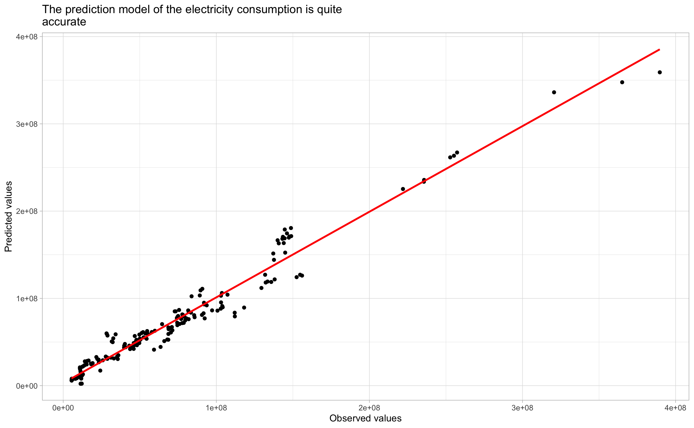This plot confirms the accuracy of our predictions.

5.1.4 Model scoring

Table 5.6: RMSE score

RMSE
12087556

Our prediction model is : Total_compsum_MWh ~ Commercial_cust + Total_generation

To conclude, we see that we need to predict the production of electricity (Total_generation) in order to be able to predict the consumption of energy (Total_compsum_MWh). This is what we will be doing in the next part.

5.2 Prediction of the electricity production

5.2.1 Training the model

We do not need to make a new PCA because the energy production is correlated to the energy consumption, thus we will thake the sames results, the same variables.

We do not take the consumption of energy in our model because we first need to predict the generation of electricity in order to predict the consumption as we have seen in the previous part. We train the following model:

Total_generation~GDP + population + house_unit + Residential_cust + Commercial_cust + Industrial_cust

We used the AIC criterion to select the best model and the house_unit variable has been removed.

Table 5.7: Total_generation ~ GDP + population + Residential_cust + Commercial_cust + Industrial_cust

Parameter	Estimate	Standard Error	P.value
(Intercept)	3131003.9	1.93e+06	0.106
GDP	-29.5	1.65e+01	0.0756
population	-25.2	2.38e+00	0 ***
Residential_cust	75.7	5.80e+00	0 ***
Commercial_cust	108.9	2.69e+01	1e-04 ***
Industrial_cust	922.9	8.12e+01	0 ***

Then we computed the VIF coefficient to check the multicollinearity.

	VIF Coefficient
GDP	25.05
population	172.92
Residential_cust	143.36
Commercial_cust	57.52
Industrial_cust	2.29

VIF coefficient of population and Residential_cust is well too high, we remove these variables.

Then we trained the following model:

Total_generation ~ GDP + Commercial_cust + Industrial_cust

Table 5.8: Total_generation ~ GDP + Commercial_cust + Industrial_cust

Parameter	Estimate	Standard Error	P.value
(Intercept)	11651946	2.02e+06	0 ***
GDP	-120	1.12e+01	0 ***
Commercial_cust	279	1.20e+01	0 ***
Industrial_cust	560	8.55e+01	0 ***

Again, we compute the VIF coefficient.

	VIF Coefficient
GDP	9.05
Commercial_cust	9.17
Industrial_cust	2.02

But the VIF coefficients were still to large for GDP (9.05) and Commercial_cust (9.17). We decided to remove the variable Commercial_cust.

Again, we train the following model:

Total_generation ~ GDP + Industrial_cust

Table 5.9: Total_generation ~ GDP + Industrial_cust

Parameter	Estimate	Standard Error	P.value
(Intercept)	33239779	2.41e+06	0 ***
GDP	109	6.95e+00	0 ***
Industrial_cust	935	1.13e+02	0 ***

Our VIF coefficients are good enough as we can see below.

	VIF Coefficient
GDP	1.94
Industrial_cust	1.94

We compute the R-Squared of the model.

Table 5.10: Total_generation ~ GDP + Industrial_cust: The R-Squared is well improved

R-Squared	Adjusted R-Squared
0.593	0.592

The R-Squared of 0.593 is really weak (Table 5.10).

In order to improve the R-Squared and instead of removing the Commercial_cust, we removed the GDP and retrained the following model:

Total_generation ~ Commercial_cust + Industrial_cust

Table 5.11: Total_generation ~ Commercial_cust + Industrial_cust

Parameter	Estimate	Standard Error	P.value
(Intercept)	17296991	2.12e+06	0 ***
Commercial_cust	164	6.04e+00	0 ***
Industrial_cust	423	9.16e+01	0 ***

	VIF Coefficient
Commercial_cust	1.97
Industrial_cust	1.97

Table 5.12: Total_generation ~ Commercial_cust + Industrial_cust: The R-Squared is well improved

R-Squared	Adjusted R-Squared
0.736	0.735

We finally found a new R-Squared of 0.736 which is much better (Table 5.12). Also, the VIF coefficients for this model are correct (< 5) so we can select the following model to predict energy production:

Total_generation ~ Commercial_cust + Industrial_cust

5.2.2 Predicting the model

In this part, we plotted the two following models and their predictions:

Total_generation ~ GDP + Industrial_cust

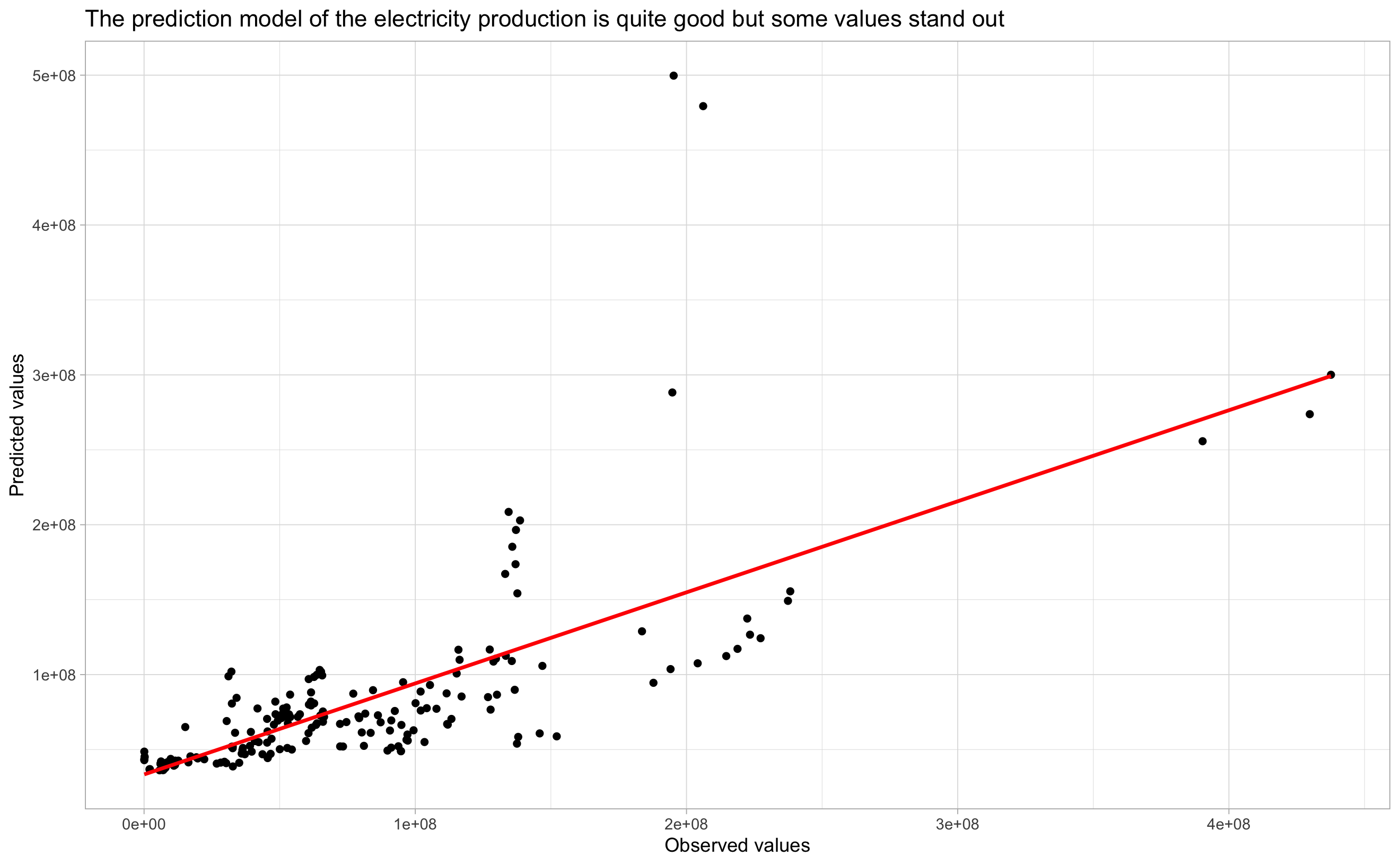
Figure 5.3: Total_generation ~ GDP + Industrial_cust

Total_generation ~ Commercial_cust + Industrial_cust

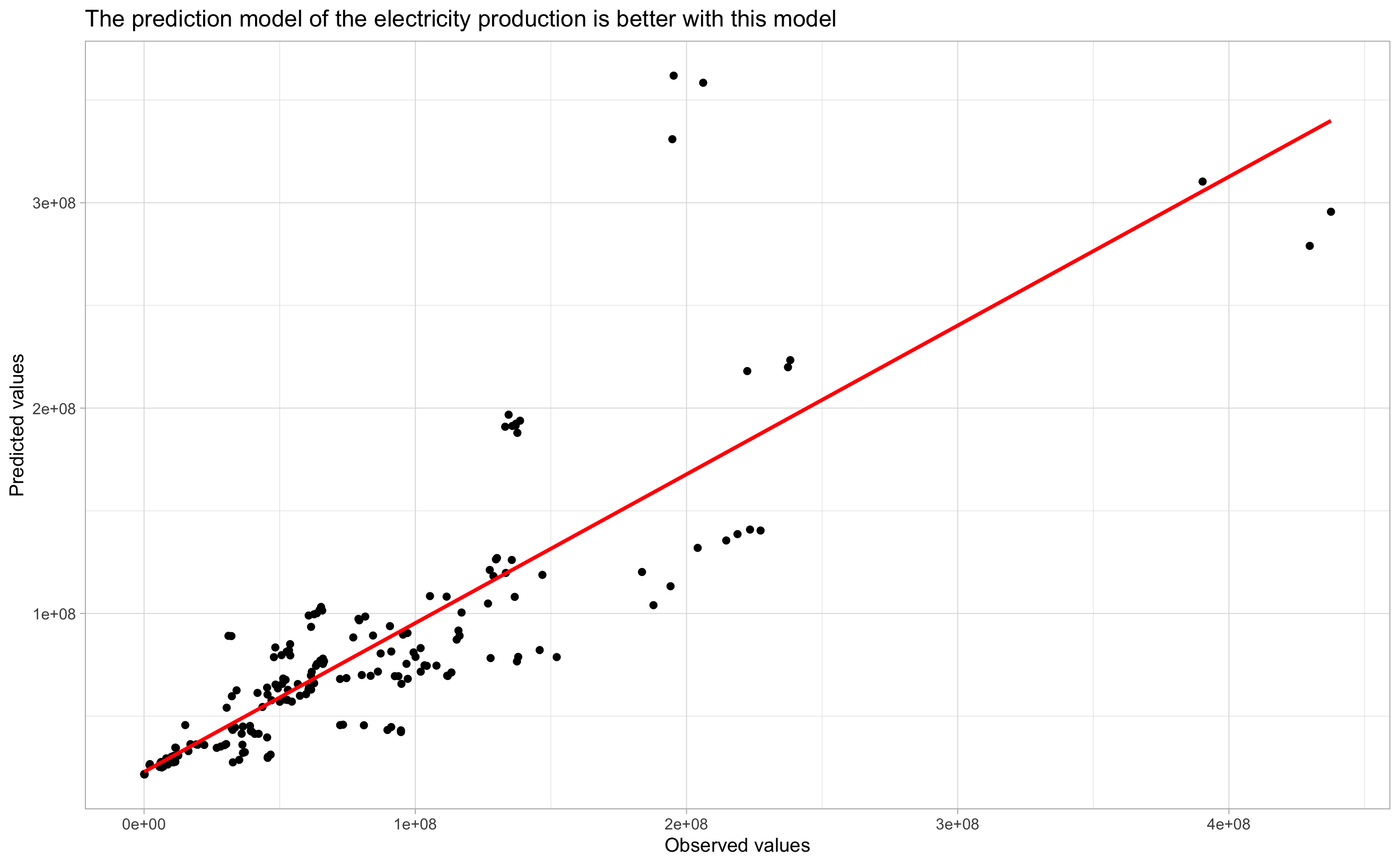
Figure 5.4: Total_generation ~ Commercial_cust + Industrial_cust

We can see that predictions are more linear in Figure 5.4 than in Figure 5.3

5.2.3 Scoring the models

We need to confirm the R-squared results by scoring the RMSE of our two models.

Table 5.13: RMSE score for Total_generation ~ GDP + Industrial_cust

RMSE
50690303

Table 5.14: RMSE score for Total_generation ~ Commercial_cust + Industrial_cust

RMSE
38050565

RMSE can confirmed the result of the R-Squared. Second model RMSE (Table 5.14) is lower than the first one (Table 5.13) so we select it.

Our final prediction model for electricity production is Total_generation ~ Commercial_cust + Industrial_cust.

Thus, the more the commercial and industrial customers, the more important is the electricity consumption.

The R-squared coefficient of our final regression (model 2) is R2 = 73.6 % (Table 5.12).

This means that our model is able to explain 73.6 % of the variations of the variable “Total_generation” in this dataset.

As a conclusion, we can say that in order to predict electricity consumption, we have to predict the electricity production. Our prediction model for energy production is less accurate than for the consumption model. Nevertheless, our models are meaningful and confirm the patterns found in the exploratory data analysis of the electricity consumption. Moreover, we could have been more accurate by choosing more variables but it would not have been possible without having a lot of multicollinearity.

5.3 Prediction of the electricity price

In this part, we will simulate the annual price of electricity by state.

First, we nested our data set with the code below :

model1_nested <- final_model %>%
  group_by(state) %>%
  nest()

region_model <- model1_nested %>%
  mutate(model = map(
    data,
    ~ lm(
      formula = price_cents_kwh ~ prop_coal + prop_gas + prop_renewable,
      data = .x
    )
  ))

We use the following variables:

• price_cents_kwh
• prop_coal
• prop_gas
• prop_renewable

For many states, the predictive capabilities of our model are very poor:

state	adj.r.squared	p.value
Hawaii	-0.033	0.494
Louisiana	-0.114	0.8364
Maine	0.136	0.1414
Maryland	0.060	0.2552
Nebraska	-0.121	0.8726
Texas	-0.086	0.6987
Rhode Island	-0.067	0.9787
District of Columbia	-0.150	0.7794

Despite a significant p.value, we also notice that several models have a very low adj.r.squared as we can see in Table 5.15. This means that the predictive power is low. Thus we arbitrarily choose to select only states with an adj.r.squared greater than 0.80.

Table 5.15: Summary of the multilinear model [p.value < 0.05]

state	adj.r.squared	p.value
Alabama	0,79	0 ***
Alaska	0,38	0.014 *
Arizona	0,42	0.0084 **
Arkansas	0,67	2e-04 ***
California	0,78	0 ***
Colorado	0,86	0 ***
Connecticut	0,47	0.0044 **
Delaware	0,71	1e-04 ***
Florida	0,69	1e-04 ***
Georgia	0,84	0 ***
Idaho	0,51	0.0026 **
Illinois	0,47	0.0044 **
Indiana	0,81	0 ***
Iowa	0,94	0 ***
Kansas	0,81	0 ***
Kentucky	0,74	0 ***
Massachusetts	0,45	0.0058 **
Michigan	0,47	0.0046 **
Minnesota	0,94	0 ***
Mississippi	0,48	0.0043 **
Missouri	0,54	0.0018 **
Montana	0,71	1e-04 ***
Nevada	0,57	0.0011 **
New Hampshire	0,65	3e-04 ***
New Jersey	0,42	0.009 **
New Mexico	0,82	0 ***
New York	0,30	0.031 *
North Carolina	0,66	2e-04 ***
North Dakota	0,90	0 ***
Ohio	0,77	0 ***
Oklahoma	0,57	0.0011 **
Oregon	0,53	0.002 **
Pennsylvania	0,88	0 ***
South Carolina	0,81	0 ***
South Dakota	0,89	0 ***
Tennessee	0,61	6e-04 ***
Utah	0,82	0 ***
Virginia	0,78	0 ***
Washington	0,74	0 ***
West Virginia	0,81	0 ***
Wisconsin	0,62	4e-04 ***
Wyoming	0,85	0 ***

In the Figure 5.5, we see that the residuals do not seem to reflect any pattern.

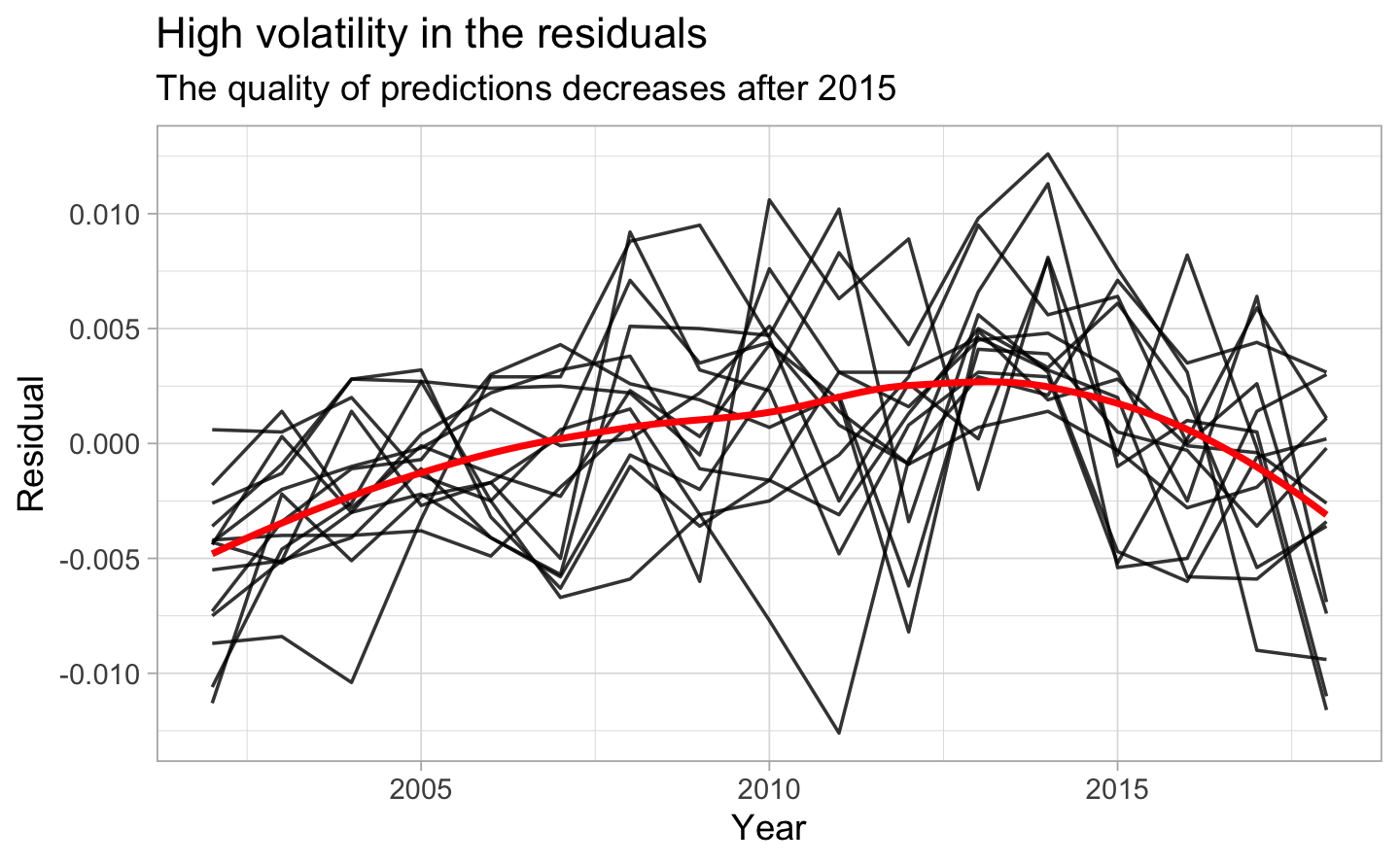
Figure 5.5: High volatility in the residuals

For these 14 states, the annual price of electricity is correctly predicted. The model reflects the upward trend of the price.

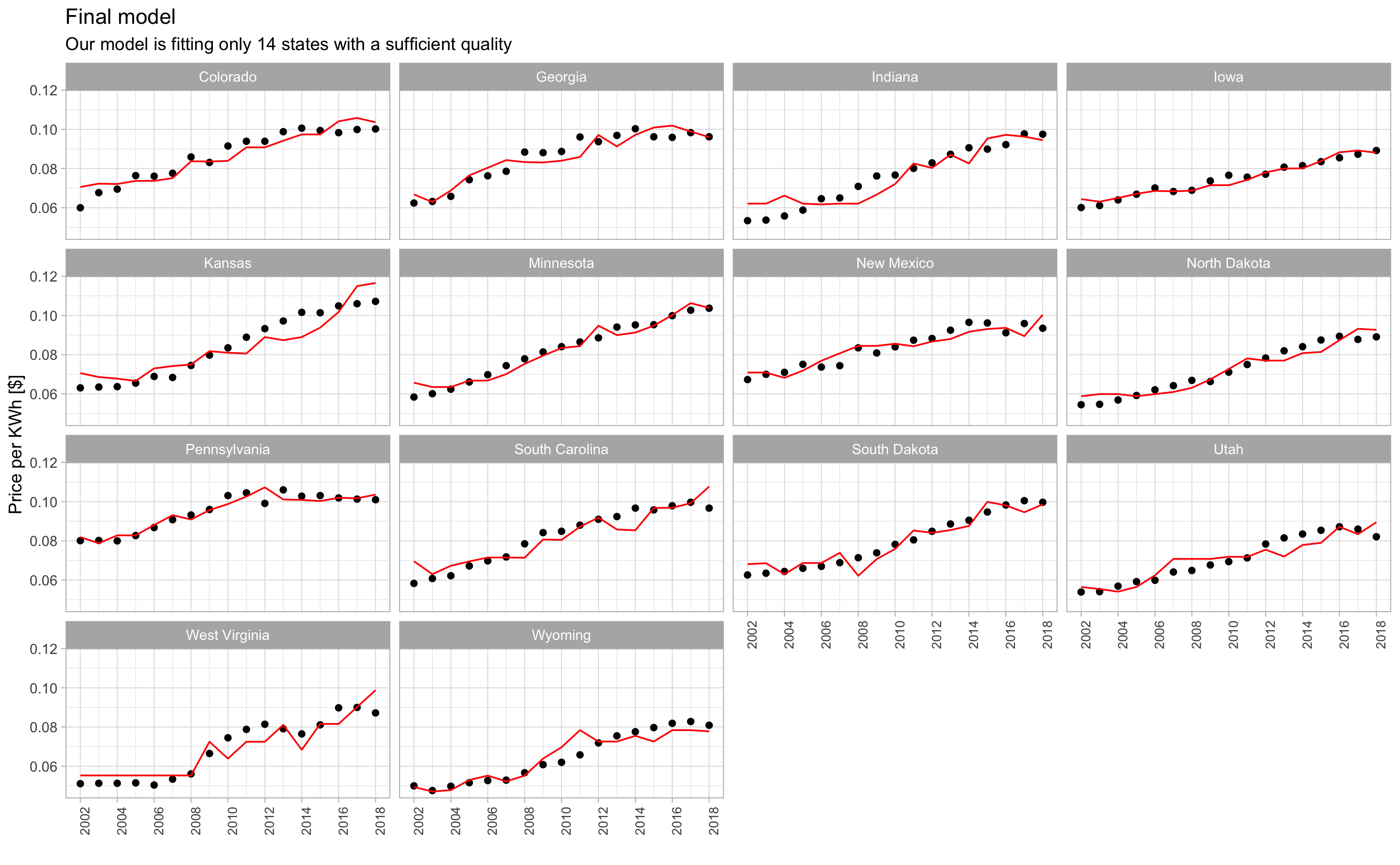
Among the states where the model succeeds in predicting the annual energy price, there is no ratio that stands out. The proportion of production is very volatile from one state to another. In addition, they belong to different regions and have different characteristics (CO2 share, population, PIB, etc.)

5.3.1 The limits of energy price prediction

We can accurately predict the annual KWh price only for some states. For the rest, either the p.value is too high or the prediction capabilities are too low. It is very difficult to predict variables in the energy field. Indeed, there are many factors that influence the price of electricity or the production (weather, economic situation, production structure, politics, etc.)

In addition, we only have access to annual data. This has severely limited our ability to make predictions. The grain used in this area of study is often in hours or minutes.

References

Abdi, Hervé, and Lynne J. Williams. 2010. “Principal Component Analysis: Principal Component Analysis.” Wiley Interdisciplinary Reviews: Computational Statistics 2 (4): 433–59. https://doi.org/10.1002/wics.101.