6 Analysis of solar and hydroelectric power generation in California
In this part we will analyse the load curves in photovoltaic and hydraulic production. We will demonstrate the differences in power between these two energies and their behaviour.
Finally, we aim to build a model that simulates power generation capacity from 2012 to 2018 and thus predict the total production.
6.1 Solar analysis
Photovoltaic panels are highly dependent on climatic factors. We will therefore see a significant seasonality on a daily and annual level.
6.1.1 Annual and monthly solar production
For the annual solar production, in Figure 6.1, we see an upward trend and a significant seasonality. The blue curve represents the average power per hour and the red curve the maximum power reached. For the months, we also notice a trend. Indeed, the total power is stronger in summer.
Finally, we can see the great volatility of solar energy. The difference between maximum and average power is significant. This is the main characteristic of renewable energies. It is also what makes their production difficult to estimate.
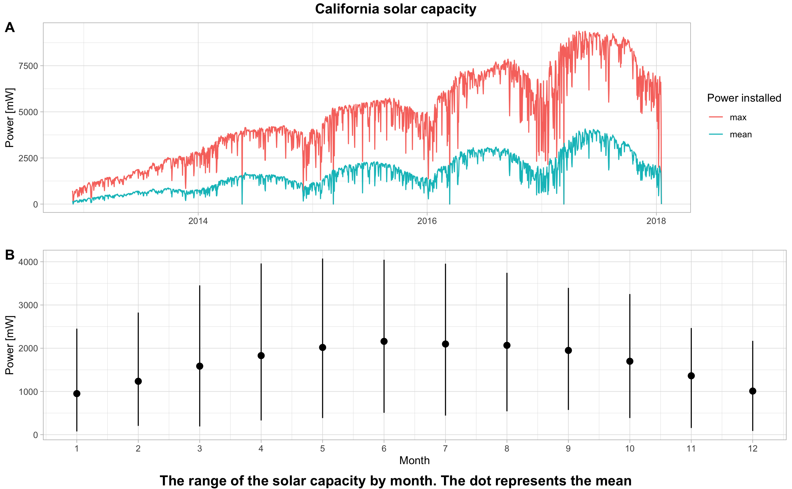
Figure 6.1: California solar capacity
6.1.2 Solar model
Our model is designed to estimate the average power per hour of the Californian photovoltaic park.
We estimate the power with the model below.
In the Table 6.1, we see the estimated coefficients, the standard deviations and the p.values.
The second coefficient is positive. Each additional year, the power increases by 525.5 mW. Finally, concerning the coefficient of the months, each additional month adds 26.9mW.
| Parameter | Estimate | Standard Error | P.value |
|---|---|---|---|
| (Intercept) | -91.8 | 39.28 | 0.0195 * |
| I(ID_year - 2012) | 525.5 | 8.77 | 0 *** |
| ID_month | 26.9 | 3.69 | 0 *** |
We clearly see that our model does not take into account the strong seasonality effect but only the upward trend.
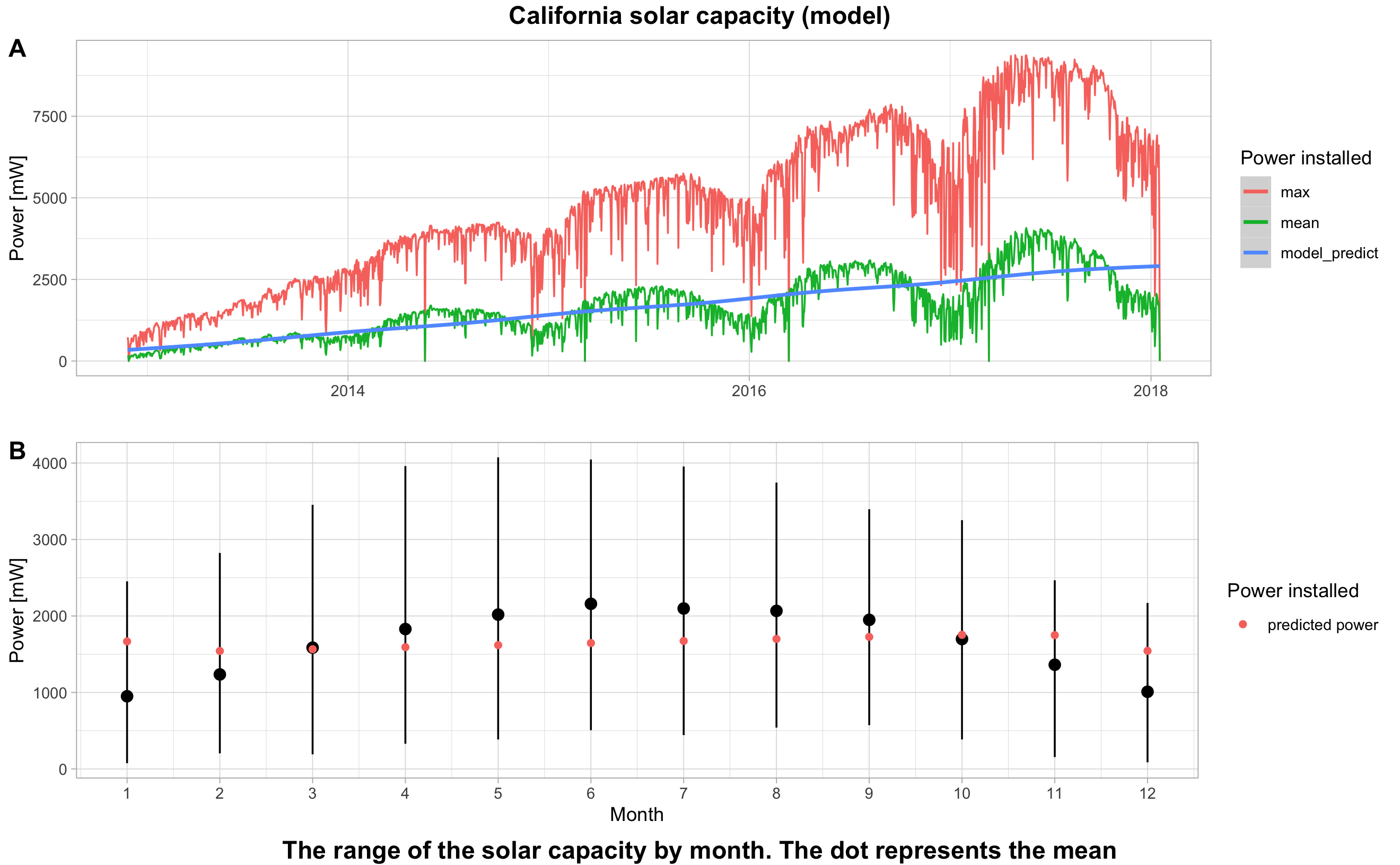
Figure 6.2: California solar capacity (model)
However, we can estimate the average production for the years in which the data were complete. In fact, by multiplying the average hourly power by 8760 hours, we obtain the total production in TWh.
6.1.3 Total solar production
| Year | Predicted generation | Observed generation |
|---|---|---|
| 2015 | 14.5 | 14.4 |
| 2016 | 19.1 | 19.4 |
| 2017 | 23.7 | 24.3 |
6.1.4 Power analysis per hour
We estimate the power with the model below which is a polynomial of order 6.
As we can see from the p.values column, all the coefficients are significant.| Coefficient | Estimate | Std. Error | t-statistic | P.value | Significance |
|---|---|---|---|---|---|
| (Intercept) | 1647 | 7 | 235.4 | 0 | *** |
| poly(ID_hour, degree = 6)1 | 29531 | 1483 | 19.9 | 0 | *** |
| poly(ID_hour, degree = 6)2 | -324651 | 1483 | -218.9 | 0 | *** |
| poly(ID_hour, degree = 6)3 | -46288 | 1483 | -31.2 | 0 | *** |
| poly(ID_hour, degree = 6)4 | 204637 | 1483 | 138.0 | 0 | *** |
| poly(ID_hour, degree = 6)5 | 30214 | 1483 | 20.4 | 0 | *** |
| poly(ID_hour, degree = 6)6 | -82282 | 1483 | -55.5 | 0 | *** |
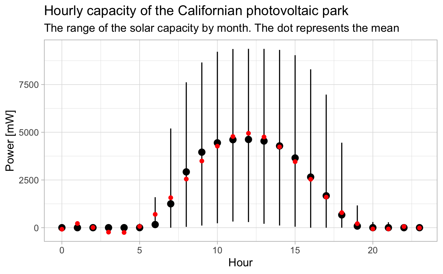
From 8:00 p.m. to 5:00 a.m., the power is obviously almost zero. During the day, the power of the solar panels has a very high volatility. This is one of the characteristics of renewable energies such as solar or wind power. They are highly dependent on climatic conditions.
However, our model fits the average hourly power pretty well.
6.2 Small hydro analysis
6.2.1 Annual and monthly solar production
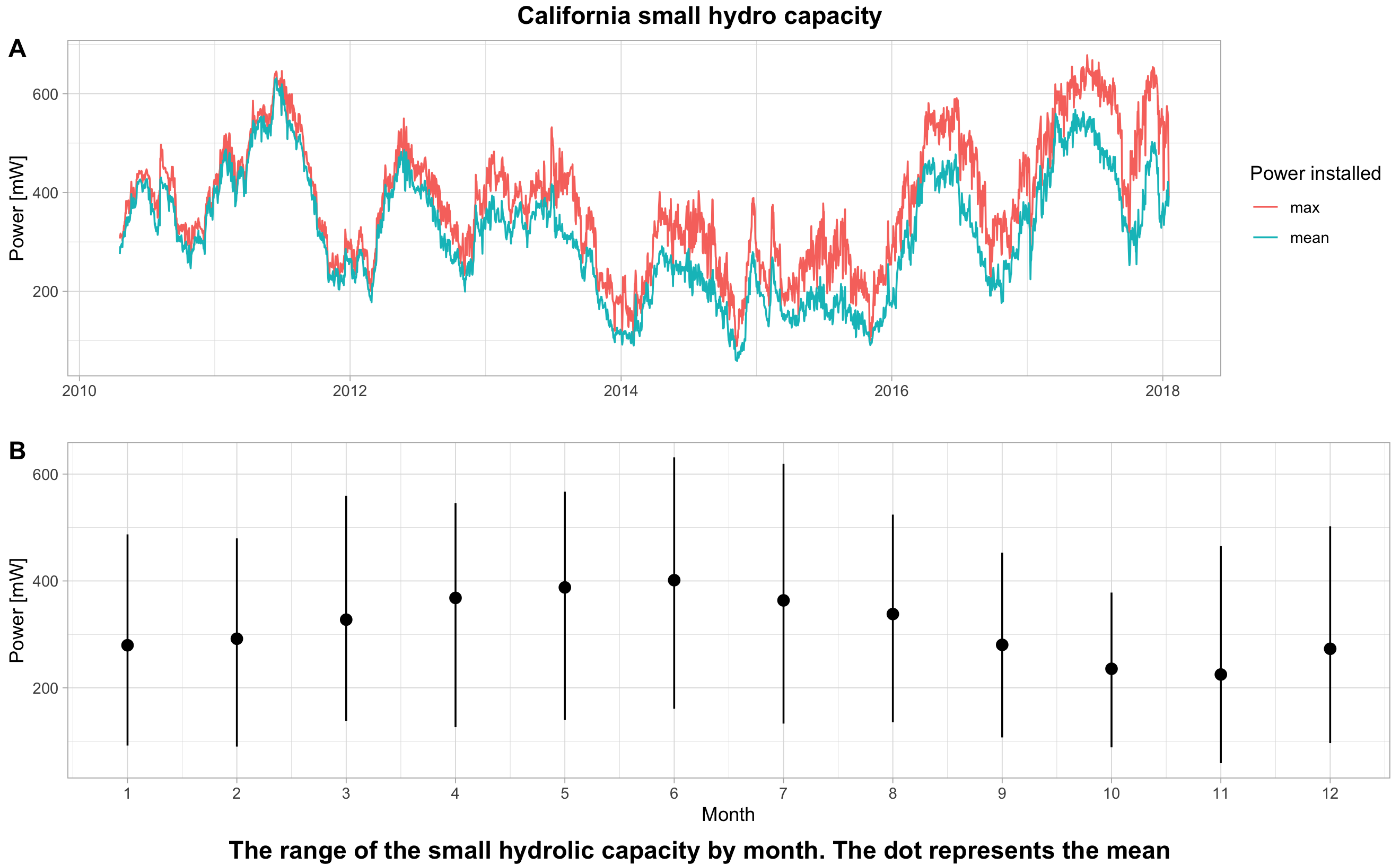
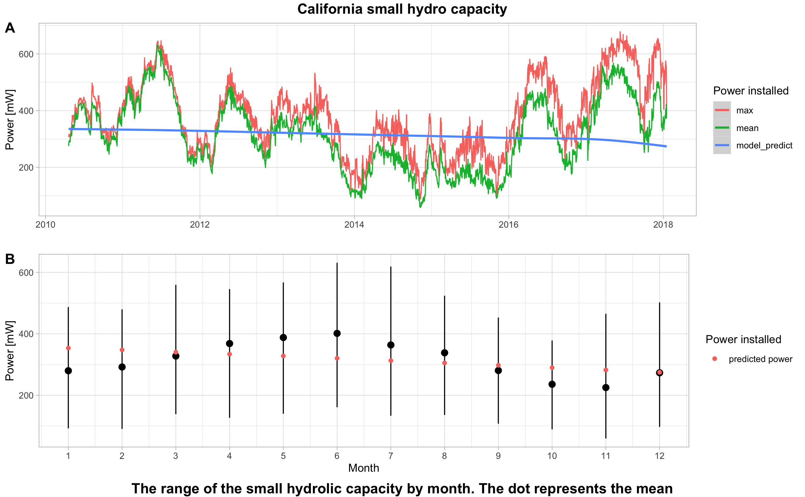
For the annual small hydro production, we can see that production varies a lot from year to year. However, there is still an annual seasonality. The blue curve represents the average power per hour and the red curve the maximum power reached. For the months, we also notice a trend. Indeed, the total power is stronger in summer.
Finally, we can demonstrate that power has a low volatility. The difference between maximum and average power is small.
In the Table 6.4, we see the estimated coefficients, the standard deviations and the p.values.
The second coefficient is negative. Each additional year, the power decreases by -6.02 mW. Finally concerning the coefficient of the months, each additional month reduces the power by -7.59 mW.| Parameter | Estimate | Standard Error | P.value |
|---|---|---|---|
| (Intercept) | 374.90 | 5.34 | 0 *** |
| I(ID_year - 2012) | -6.02 | 1.01 | 0 *** |
| ID_month | -7.59 | 0.66 | 0 *** |
We clearly see that our model does not take into account the strong seasonality effect.
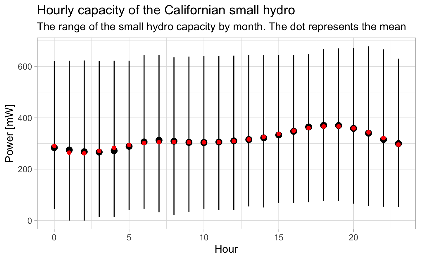
6.2.2 Power analysis per hour
We estimate the power with the model below which is a polynomial of order 6.
As we can see from the p.values column, all the coefficients are significant.
| Coefficient | Estimate | Std. Error | t-statistic | P.value | Significance |
|---|---|---|---|---|---|
| (Intercept) | 314 | 0.488 | 643.9 | 0 | *** |
| poly(ID_hour, degree = 6)1 | 6213 | 126.865 | 49.0 | 0 | *** |
| poly(ID_hour, degree = 6)2 | -2060 | 126.865 | -16.2 | 0 | *** |
| poly(ID_hour, degree = 6)3 | -3102 | 126.865 | -24.4 | 0 | *** |
| poly(ID_hour, degree = 6)4 | -2009 | 126.865 | -15.8 | 0 | *** |
| poly(ID_hour, degree = 6)5 | -1837 | 126.865 | -14.5 | 0 | *** |
| poly(ID_hour, degree = 6)6 | 1711 | 126.865 | 13.5 | 0 | *** |
The power of the small hydro is constant throughout the day. This is the major difference with renewable energy (solar or wind).
Our model fits the average hourly power pretty well.
6.3 The limits of our model
Our series are not stationary. We should therefore have applied a model that takes seasonality into account. In order to deepen this analysis and to better predict the load curves, it would be interesting to apply an ARIMA model for example or exponential smoothing techniques.
In addition, in order to predict the future production of solar and wind power, it is essential to collect external weather data. However, we can already demonstrate the behaviour of the different load curves regarding the type of energy.
On the one hand, renewable energies will be very volatile and therefore more difficult to predict (solar, wind). On the other hand, traditional energies (coal, gas and hydraulic) are not very volatile and therefore more easily predictable.