Chapter 5 Spatial Analysis
5.1 Processing
rm(list = ls())
library(tidyverse)
library(spdep)
library(tmap)
library(sf)
library(leaflet)

dat_ci_map <- readRDS("./_dat/dat_ci_map_v3.rds") %>%
  filter(sample.size>=10) %>%
  filter(rii !=Inf & rii>0)
dat_edu_map <- readRDS("./_dat/dat_edu_map_v2.rds") %>%
  filter(sample.size>=10) %>%
  filter(rii !=Inf & rii>0)
source("./mal_ineq_fun.R")

breaks <- c(-Inf, -2.58, -1.96, -1.65, 1.65, 1.96, 2.58, Inf)
labels <- c("Cold spot: 99% confidence", "Cold spot: 95% confidence", "Cold spot: 90% confidence", "PSU Not significant","Hot spot: 90% confidence", "Hot spot: 95% confidence", "Hot spot: 99% confidence")

library(spData)
sPDF <- world %>%
  filter(continent == "Africa")
5.2 Wealth
dat_ci_sp <- as(dat_ci_map, "Spatial")

coords<-coordinates(dat_ci_sp)
IDs<-row.names(as.data.frame(coords))
Neigh_nb<-knn2nb(knearneigh(coords, k=1, longlat = TRUE), row.names=IDs)
dsts<-unlist(nbdists(Neigh_nb,coords))
max_1nn<-max(dsts)
Neigh_kd1<-dnearneigh(coords,d1=0, d2=max_1nn, row.names=IDs)

self<-nb2listw(Neigh_kd1, style="W", zero.policy = T)

w.getis <- dat_ci_map %>%
  st_set_geometry(NULL) %>%
  nest() %>%
  crossing(var1 = c("ci_val", "sii", "rii")) %>%
  mutate(data_sub = map2(.x = data, .y = var1, .f = ~dplyr::select(.x, .y, country, cluster_number,
                                                                   prev, lat, long) %>%
                           rename(output = 1)),
         LISA = map(.x = data_sub, .f = ~localG(.x$output, self)),
         clust_LISA = map(.x = LISA, .f = ~cut(.x, include.lowest = TRUE,
                                               breaks = breaks, labels = labels))) %>%
  dplyr::select(data_sub, var1, LISA, clust_LISA) %>%
  unnest()
5.2.1 W-CI
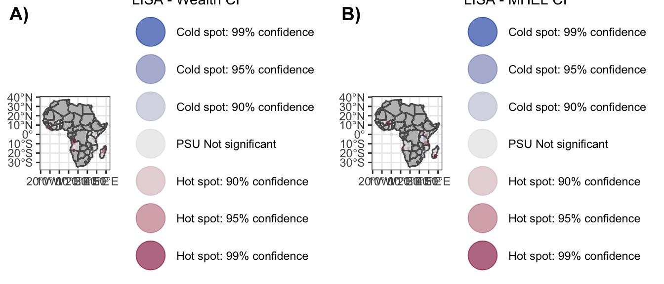
Supplementary Figure 13_a
dat_w_map_ci <- w.getis %>%
  filter(var1 =="ci_val") %>%
  st_as_sf(coords = c("long", "lat"), crs = 4326) %>%
  filter(!is.na(LISA)) %>%
  dplyr::mutate(lat = sf::st_coordinates(.)[,2],
                long = sf::st_coordinates(.)[,1])

pal <- colorFactor("RdBu", dat_w_map_ci$clust_LISA, reverse = T)

# dat_w_map_ci %>%
#   leaflet() %>%
#   addTiles() %>%
#   addCircles(lng = ~long, lat = ~lat, color = ~ pal(clust_LISA),
#              popup = paste("Country", dat_w_map_ci$country, "<br>",
#                            "Cluster:", dat_w_map_ci$cluster_number, "<br>",
#                            "Malaria Prevalence:", dat_w_map_ci$prev, "<br>",
#                            "CI:", dat_w_map_ci$output, "<br>",
#                            "LISA:", dat_w_map_ci$LISA)) %>%
#   addLegend("bottomright",
#             pal = pal, values = ~clust_LISA,
#             title = "LISA - Wealth CI") %>%
#   addScaleBar(position = c("bottomleft"))

sf13_a <- ggplot() +
  geom_sf(data = sPDF, fill = "grey") +
  geom_sf(data = dat_w_map_ci,
          aes(col = clust_LISA), size = .5, alpha =.6) +
  geom_sf(data = sPDF, fill = NA) +
  scale_color_discrete_diverging(palette = "Blue-Red",
                                 limits = labels) +
  labs(color = "LISA - Wealth CI") +
  guides(colour = guide_legend(override.aes = list(size=10))) +
  theme_bw()
5.2.2 W-SII
Figure 3_a
dat_w_map_sii <- w.getis %>%
  filter(var1 =="sii") %>%
  st_as_sf(coords = c("long", "lat"), crs = 4326) %>%
  filter(!is.na(LISA)) %>%
  dplyr::mutate(lat = sf::st_coordinates(.)[,2],
                long = sf::st_coordinates(.)[,1])

pal <- colorFactor("RdBu", dat_w_map_sii$clust_LISA, reverse = T)

# dat_w_map_sii %>%
#   leaflet() %>%
#   addTiles() %>%
#   addCircles(lng = ~long, lat = ~lat, color = ~ pal(clust_LISA),
#              popup = paste("Country", dat_w_map_sii$country, "<br>",
#                            "Cluster:", dat_w_map_sii$cluster_number, "<br>",
#                            "Malaria Prevalence:", dat_w_map_sii$prev, "<br>",
#                            "CI:", dat_w_map_sii$output, "<br>",
#                            "LISA:", dat_w_map_sii$LISA)) %>%
#   addLegend("bottomright",
#             pal = pal, values = ~clust_LISA,
#             title = "LISA - Wealth SII") %>%
#   addScaleBar(position = c("bottomleft"))

f3_a <- ggplot() +
  geom_sf(data = sPDF, fill = "grey") +
  geom_sf(data = dat_w_map_sii,
          aes(col = clust_LISA), size = .5, alpha =.6) +
  geom_sf(data = sPDF, fill = NA) +
  scale_color_discrete_diverging(palette = "Blue-Red",
                                 limits = labels) +
  labs(color = "LISA - Wealth SII") +
  guides(colour = guide_legend(override.aes = list(size=10))) +
  theme_bw()
5.2.3 W-RII
Figure 3_b
dat_w_map_rii <- w.getis %>%
  filter(var1 =="rii") %>%
  st_as_sf(coords = c("long", "lat"), crs = 4326) %>%
  filter(!is.na(LISA)) %>%
  dplyr::mutate(lat = sf::st_coordinates(.)[,2],
                long = sf::st_coordinates(.)[,1])

pal <- colorFactor("RdBu", dat_w_map_rii$clust_LISA, reverse = T)

# dat_w_map_rii %>%
#   leaflet() %>%
#   addTiles() %>%
#   addCircles(lng = ~long, lat = ~lat, color = ~ pal(clust_LISA),
#              popup = paste("Country", dat_w_map_rii$country, "<br>",
#                            "Cluster:", dat_w_map_rii$cluster_number, "<br>",
#                            "Malaria Prevalence:", dat_w_map_rii$prev, "<br>",
#                            "CI:", dat_w_map_rii$output, "<br>",
#                            "LISA:", dat_w_map_rii$LISA)) %>%
#   addLegend("bottomright",
#             pal = pal, values = ~clust_LISA,
#             title = "LISA - Wealth RII") %>%
#   addScaleBar(position = c("bottomleft"))

f3_b <- ggplot() +
  geom_sf(data = sPDF, fill = "grey") +
  geom_sf(data = dat_w_map_rii,
          aes(col = clust_LISA), size = .5, alpha =.6) +
  geom_sf(data = sPDF, fill = NA) +
  scale_color_discrete_diverging(palette = "Blue-Red",
                                 limits = labels) +
  labs(color = "LISA - Wealth RII") +
  guides(colour = guide_legend(override.aes = list(size=10))) +
  theme_bw()
5.3 Education
dat_edu_sp <- as(dat_edu_map, "Spatial")

coords<-coordinates(dat_edu_sp)
IDs<-row.names(as.data.frame(coords))
Neigh_nb<-knn2nb(knearneigh(coords, k=1, longlat = TRUE), row.names=IDs)
dsts<-unlist(nbdists(Neigh_nb,coords))
max_1nn<-max(dsts)
Neigh_kd1<-dnearneigh(coords,d1=0, d2=max_1nn, row.names=IDs)

self<-nb2listw(Neigh_kd1, style="W", zero.policy = T)

w.getis_e <- dat_edu_map %>%
  st_set_geometry(NULL) %>%
  nest() %>%
  crossing(var1 = c("ci_val", "sii", "rii")) %>%
  mutate(data_sub = map2(.x = data, .y = var1, .f = ~dplyr::select(.x, .y, country, cluster_number,
                                                                   prev, lat, long) %>%
                           rename(output = 1)),
         LISA = map(.x = data_sub, .f = ~localG(.x$output, self)),
         clust_LISA = map(.x = LISA, .f = ~cut(.x, include.lowest = TRUE,
                                               breaks = breaks, labels = labels))) %>%
  dplyr::select(data_sub, var1, LISA, clust_LISA) %>%
  unnest()
5.3.1 E-CI
Supplementary Figure 13_b
dat_e_map_ci <- w.getis_e %>%
  filter(var1 =="ci_val") %>%
  st_as_sf(coords = c("long", "lat"), crs = 4326) %>%
  filter(!is.na(LISA)) %>%
  dplyr::mutate(lat = sf::st_coordinates(.)[,2],
                long = sf::st_coordinates(.)[,1])

pal <- colorFactor("RdBu", dat_e_map_ci$clust_LISA, reverse = T)

# dat_e_map_ci %>%
#   leaflet() %>%
#   addTiles() %>%
#   addCircles(lng = ~long, lat = ~lat, color = ~ pal(clust_LISA),
#              popup = paste("Country", dat_e_map_ci$country, "<br>",
#                            "Cluster:", dat_e_map_ci$cluster_number, "<br>",
#                            "Malaria Prevalence:", dat_e_map_ci$prev, "<br>",
#                            "CI:", dat_e_map_ci$output, "<br>",
#                            "LISA:", dat_e_map_ci$LISA)) %>%
#   addLegend("bottomright",
#             pal = pal, values = ~clust_LISA,
#             title = "LISA - Education CI") %>%
#   addScaleBar(position = c("bottomleft"))

sf13_b <- ggplot() +
  geom_sf(data = sPDF, fill = "grey") +
  geom_sf(data = dat_e_map_ci,
          aes(col = clust_LISA), size = .5, alpha =.6) +
  geom_sf(data = sPDF, fill = NA) +
  scale_color_discrete_diverging(palette = "Blue-Red",
                                 limits = labels) +
  labs(color = "LISA - MHEL CI") +
  guides(colour = guide_legend(override.aes = list(size=10))) +
  theme_bw()
5.3.2 E-SII
Figure 3_c
dat_e_map_sii <- w.getis_e %>%
  filter(var1 =="sii") %>%
  st_as_sf(coords = c("long", "lat"), crs = 4326) %>%
  filter(!is.na(LISA)) %>%
  dplyr::mutate(lat = sf::st_coordinates(.)[,2],
                long = sf::st_coordinates(.)[,1])

pal <- colorFactor("RdBu", dat_e_map_sii$clust_LISA, reverse = T)

# dat_e_map_sii %>%
#   leaflet() %>%
#   addTiles() %>%
#   addCircles(lng = ~long, lat = ~lat, color = ~ pal(clust_LISA),
#              popup = paste("Country", dat_e_map_sii$country, "<br>",
#                            "Cluster:", dat_e_map_sii$cluster_number, "<br>",
#                            "Malaria Prevalence:", dat_e_map_sii$prev, "<br>",
#                            "CI:", dat_e_map_sii$output, "<br>",
#                            "LISA:", dat_e_map_sii$LISA)) %>%
#   addLegend("bottomright",
#             pal = pal, values = ~clust_LISA,
#             title = "LISA - Education SII") %>%
#   addScaleBar(position = c("bottomleft"))

f3_c <- ggplot() +
  geom_sf(data = sPDF, fill = "grey") +
  geom_sf(data = dat_e_map_sii,
          aes(col = clust_LISA), size = .5, alpha =.6) +
  geom_sf(data = sPDF, fill = NA) +
  scale_color_discrete_diverging(palette = "Blue-Red",
                                 limits = labels) +
  labs(color = "LISA - MHEL SII") +
  guides(colour = guide_legend(override.aes = list(size=10))) +
  theme_bw()
5.3.3 E-RII
Figure 3_d
dat_e_map_rii <- w.getis_e %>%
  filter(var1 =="rii") %>%
  st_as_sf(coords = c("long", "lat"), crs = 4326) %>%
  filter(!is.na(LISA)) %>%
  dplyr::mutate(lat = sf::st_coordinates(.)[,2],
                long = sf::st_coordinates(.)[,1])

pal <- colorFactor("RdBu", dat_e_map_rii$clust_LISA, reverse = T)

# dat_e_map_rii %>%
#   leaflet() %>%
#   addTiles() %>%
#   addCircles(lng = ~long, lat = ~lat, color = ~ pal(clust_LISA),
#              popup = paste("Country", dat_e_map_rii$country, "<br>",
#                            "Cluster:", dat_e_map_rii$cluster_number, "<br>",
#                            "Malaria Prevalence:", dat_e_map_rii$prev, "<br>",
#                            "CI:", dat_e_map_rii$output, "<br>",
#                            "LISA:", dat_e_map_rii$LISA)) %>%
#   addLegend("bottomright",
#             pal = pal, values = ~clust_LISA,
#             title = "LISA - Education RII") %>%
#   addScaleBar(position = c("bottomleft"))

f3_d <- ggplot() +
  geom_sf(data = sPDF, fill = "grey") +
  geom_sf(data = dat_e_map_rii,
          aes(col = clust_LISA), size = .5, alpha =.6) +
  geom_sf(data = sPDF, fill = NA) +
  scale_color_discrete_diverging(palette = "Blue-Red",
                                 limits = labels) +
  labs(color = "LISA - MHEL RII") +
  guides(colour = guide_legend(override.aes = list(size=10))) +
  theme_bw()
5.4 Figures
library(cowplot)

(f3 <- plot_grid(f3_a, f3_b, f3_c, f3_d,
                 labels = c("A)", "B)", "C)", "D)"),
                 ncol = 2))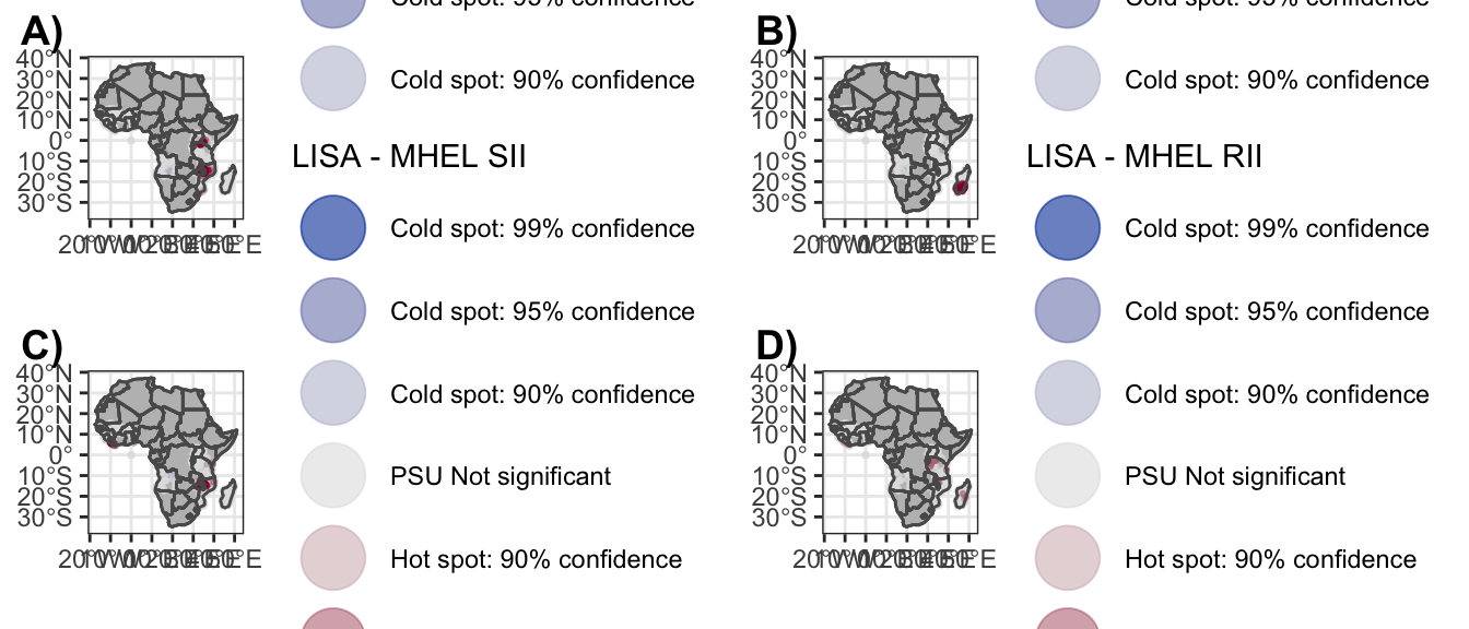
5.5 Summary Table
dat.ci <- readRDS("./_dat/dat_ci.rds") %>%
  #st_set_geometry(NULL) %>%
  group_by(country) %>%
  summarise(#wealth = median(wealth, na.rm = T),
         sample_w = sum(sample.size, na.rm = T),
         prev_w = median(prev, na.rm = T),
         sii_w = median(sii, na.rm = T),
         rii_w = median(rii, na.rm = T)
         )

dat.edu <- readRDS("./_dat/dat_edu.rds") %>%
  #st_set_geometry(NULL) %>%
  group_by(country) %>%
  summarise(#wealth = median(wealth, na.rm = T),
         sample_e = sum(sample.size, na.rm = T),
         prev_e = median(prev, na.rm = T),
         sii_e = median(sii, na.rm = T),
         rii_e = median(rii, na.rm = T)
         )

dat <- dat.ci %>%
  left_join(dat.edu, by = "country")

dat
## # A tibble: 13 x 9
## country sample_w prev_w sii_w rii_w sample_e prev_e sii_e rii_e
## <chr> <int> <dbl> <dbl> <dbl> <int> <dbl> <dbl> <dbl>
## 1 AO 1199 0.222 -0.0138 0.944 822 0.222 0.00335 1.01
## 2 BF 4954 0.2 0.0539 1.46 4046 0.2 0.156 3.83
## 3 BU 2099 0.167 0.0534 1.46 1923 0.175 0.154 3.16
## 4 KE 4318 0.162 0.0829 1.60 913 0.2 0.157 3.16
## 5 LB 2685 0.530 0.0896 1.22 1909 0.529 0.197 1.61
## 6 MD 1947 0.0808 0.0632 3.11 1355 0.0934 0.0271 1.63
## 7 ML 6534 0.318 0.0405 1.13 5217 0.3 0.0923 2.03
## 8 MW 1840 0.333 0.200 2.21 1332 0.357 0.222 2.76
## 9 MZ 3430 0.437 0.131 1.50 2821 0.452 0.109 1.40
## 10 SL 7406 0.6 0.0637 1.11 4282 0.6 0.0843 1.17
## 11 TG 2831 0.470 0.0535 1.12 2426 0.453 0.0924 1.34
## 12 TZ 2942 0.133 0.129 2.18 2188 0.143 0.114 1.92
## 13 UG 5219 0.261 0.0716 1.39 3953 0.3 0.0857 1.63