Chapter 4 Analysis Education
4.1 Processing - Education
rm(list = ls())
library(IC2)
library(codebook)
library(tidyverse)

dat <- read.csv("./_dat/dat_mal_ineq_v3.csv")
source("./mal_ineq_fun.R")

# epiDisplay::tab1(dat$rapid_test)
# epiDisplay::tab1(dat$mothers_highest_educational_level)
# epiDisplay::tab1(dat$education)
# epiDisplay::tab1(dat$edu)

#codebook_browser(dat)

# ==== NOT RUN =======
# ao <- dat %>%
#   filter(country == "SN") %>%
#   dplyr::select(rapid_test, edu, w) %>%
#   filter(complete.cases(.))
#
# ao_ci <- IC2::calcSConc(x = ao$rapid_test,
#                         y = ao$edu,
#                         w = ao$w)
# ==== NOT RUN =======

dat.n <- dat %>%
  group_by(country, REGNAME, cluster_number) %>%
  nest() %>%
  mutate(sample.size.N = map(.x = data, .f = ~dplyr::select(.x, rapid_test, edu, w) %>%
                               count(name = "N") %>% unlist()),
         sample.size.m = map(.x = data, .f = ~dplyr::select(.x, rapid_test, edu, w) %>%
                               filter(!is.na(rapid_test)) %>%
                               count(name = "N_m") %>% unlist()),
         dat_s = map(.x = data, .f = ~dplyr::select(.x, rapid_test, edu, w) %>%
                       filter(complete.cases(.))),
         sample.size = map(.x = dat_s, .f = ~count(.x) %>% unlist()),
         prev = map(.x = dat_s, .f = ~mean(.x$rapid_test, na.rm=T)),
         edu_cats = map(.x = dat_s, .f = ~distinct(.x, edu) %>% nrow())) %>%
  # FILTERS =======================
  filter(prev > 0 & prev < 1) %>%
  filter(sample.size>=10) %>%
  filter(edu_cats>1)

dat_edu.n <- dat.n  %>%
  mutate(ci = map(.x = dat_s, .f = ~IC2::calcSConc(x = .x$rapid_test,
                        y = .x$edu,
                        w = .x$w)),
         ci_val = map(.x = ci, .f = ~.x$ineq$index),
         h_calc = map(.x = dat_s, .f = ~h_ineq(dat = .x, var_soc = edu, var_outcome = rapid_test))
         )

dat_edu <- dat_edu.n %>%
  dplyr::select(country, cluster_number, sample.size.N, sample.size.m, sample.size, prev, edu_cats, ci_val, h_calc) %>%
  unnest() %>%
  ungroup()

# Checks ========
dat_edu %>%
  ggplot(aes(x=c_index, y = ci_val)) +
  geom_point(alpha = .4) +
  labs(x = "hand calculation", y = "package calculation")

# ==== NOT RUN =======
# unique(dat.n$country)
# unique(dat_ci$country)
#
# range(dat$w)
# range(dat_ci$N_m)
# range(dat_ci$n)
# range(dat_ci$ci_val, na.rm = T)
#
# hist(dat_ci$N_m)
# hist(dat_ci$n)
# hist(dat_ci$ci_val)
# ==== NOT RUN =======

#saveRDS(dat_edu, "./_dat/dat_edu.rds")
4.2 Spatial data - Education
library(sf)
library(leaflet)
library(stringr)

dat_edu_map <- dat_edu %>%
  inner_join(read.csv("./_dat/dat_gps_flat.csv"), by = c("country", "cluster_number")) %>%
  st_as_sf(coords = c("LONGNUM", "LATNUM"), crs = 4326) %>%
  dplyr::mutate(lat = sf::st_coordinates(.)[,2],
                long = sf::st_coordinates(.)[,1])

#saveRDS(dat_edu_map, "./_dat/dat_edu_map_v2.rds")

dat_adm <- dat_edu %>%
  group_by(country, REGNAME) %>%
  summarise(N = sum(sample.size.N, na.rm = T),
            N_m = sum(sample.size.m, na.rm = T),
            n = sum(sample.size, na.rm = T),
            prev = median(prev, na.rm = T),
            ci_val = median(ci_val, na.rm = T),
            sii = median(sii, na.rm = T),
            rii = median(rii, na.rm = T))

dat_edu_adm <- st_read("./_dat/SHP/union/DHS_adm.shp") %>%
  inner_join(dat_adm, by = c("country", "REGNAME"))
## Reading layer `DHS_adm' from data source `/Users/gabrielcarrasco/Dropbox/Work/Tarik LAB/Malaria Ineq/mal_ineq/_dat/SHP/union/DHS_adm.shp' using driver `ESRI Shapefile'
## Simple feature collection with 147 features and 3 fields
## Geometry type: MULTIPOLYGON
## Dimension: XY
## Bounding box: xmin: -13.30198 ymin: -26.86819 xmax: 50.49459 ymax: 15.7047
## Geodetic CRS: WGS 844.3 CI - Education
4.3.1 Plots CI -Education
Supplementary Figure 12
library(cowplot)

ci_box_10 <- dat_edu_map %>% filter(sample.size>=10) %>% ci_box(var = ci_val)
ci_box_20 <- dat_edu_map %>% filter(sample.size>=20) %>% ci_box(var = ci_val)
ci_box_30 <- dat_edu_map %>% filter(sample.size>=30) %>% ci_box(var = ci_val)

ci_box1 <- plot_grid(ci_box_10, ci_box_20, ci_box_30, labels = c("A)", "B)", "C)"), ncol = 1)

ci_prev_10 <- dat_edu_map %>% filter(sample.size>=10) %>% ci_prev(var = ci_val)
ci_prev_20 <- dat_edu_map %>% filter(sample.size>=20) %>% ci_prev(var = ci_val)
ci_prev_30 <- dat_edu_map %>% filter(sample.size>=30) %>% ci_prev(var = ci_val)

ci_prev1 <- plot_grid(ci_prev_10, ci_prev_20, ci_prev_30, labels = c("A)", "B)", "C)"), ncol = 1)

(sf12 <- plot_grid(ci_box1, ci_prev1, ncol = 2))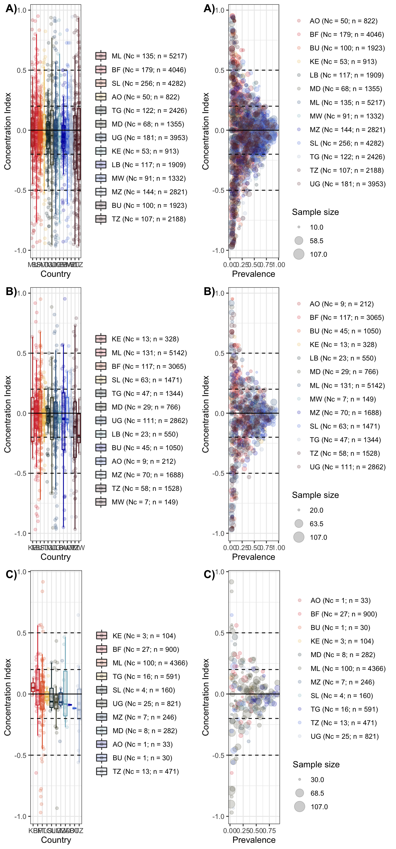
4.3.2 Maps CI - Education
Supplementary Figure 11
# library(mapview)
#
# m1 <- dat_edu_map %>%
#   filter(!is.na(ci_val)) %>%
#   mapview(zcol = "ci_val", legend = TRUE, layer.name = "CI (psu)")
#
# m2 <- dat_edu_adm %>%
#   mapview(zcol = "ci_val", legend = TRUE, layer.name = "CI (Adm)")
#
# m1 + m2

library(colorspace)

sf11_a <- ggplot() +
  geom_sf(data = sPDF, fill = "grey") +
  geom_sf(data = dat_edu_map %>%
            filter(!is.na(ci_val)),
          aes(col = ci_val), size = .5, alpha =.6) +
  geom_sf(data = sPDF, fill = NA) +
  scale_color_continuous_diverging(palette = "Tropic") +
  labs(color = "CI") +
  theme_bw()

sf11_b <- ggplot() +
  geom_sf(data = sPDF, fill = "grey") +
  geom_sf(data = dat_edu_adm, aes(fill = ci_val),
          size = 0) +
  geom_sf(data = sPDF, fill = NA) +
  scale_fill_continuous_diverging(palette = "Tropic") +
  labs(fill = "CI") +
  theme_bw()

(sf11 <- plot_grid(sf11_a, sf11_b, ncol = 2,
                  labels = c("A)","B)")))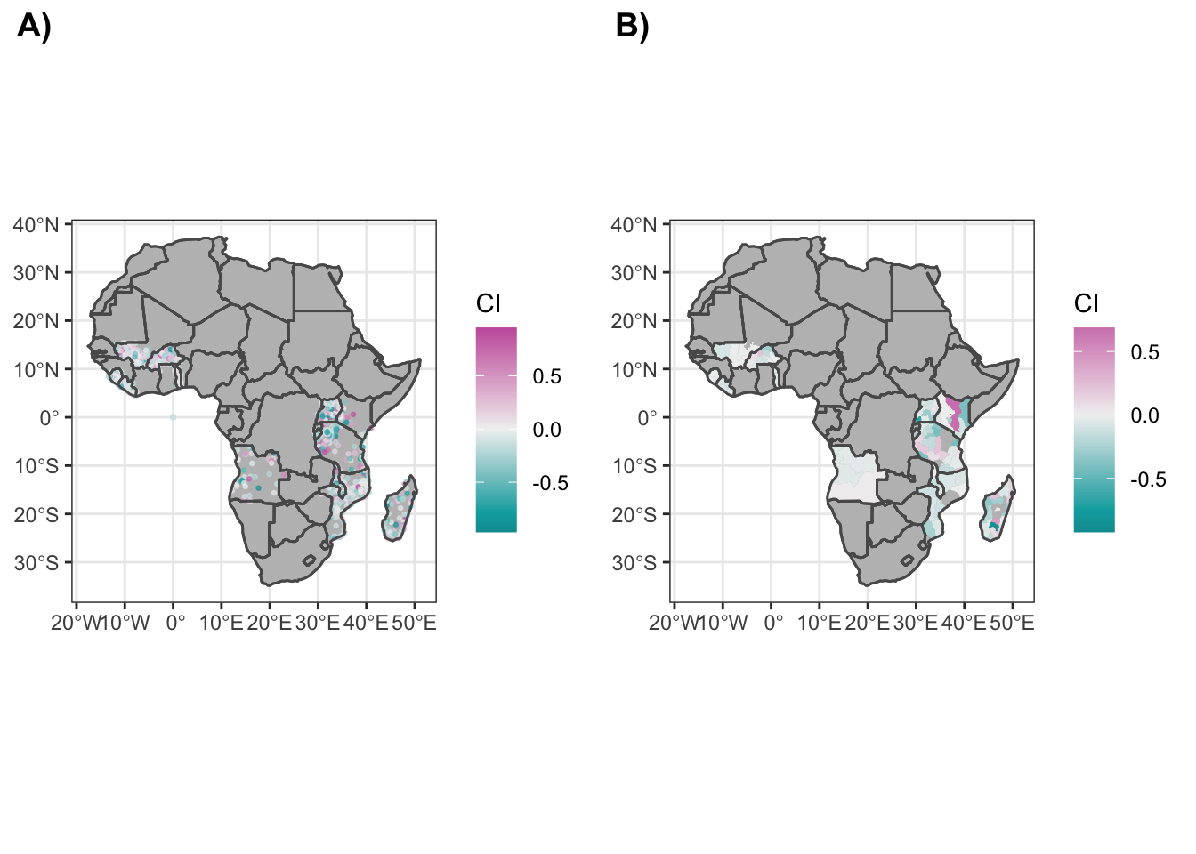
4.4 SII - Education
4.4.1 Plots SII - Education
Supplementary Figure 04
library(cowplot)

sii_box_10 <- dat_edu_map %>% filter(sample.size>=10) %>% ci_box(var = sii, y_lab = "SII")
sii_box_20 <- dat_edu_map %>% filter(sample.size>=20) %>% ci_box(var = sii, y_lab = "SII")
sii_box_30 <- dat_edu_map %>% filter(sample.size>=30) %>% ci_box(var = sii, y_lab = "SII")

sii_box <- plot_grid(sii_box_10, sii_box_20, sii_box_30, labels = c("A)", "B)", "C)"), ncol = 1)

sii_prev_10 <- dat_edu_map %>% filter(sample.size>=10) %>% ci_prev(var = sii, y_lab = "SII")
sii_prev_20 <- dat_edu_map %>% filter(sample.size>=20) %>% ci_prev(var = sii, y_lab = "SII")
sii_prev_30 <- dat_edu_map %>% filter(sample.size>=30) %>% ci_prev(var = sii, y_lab = "SII")

sii_prev <- plot_grid(sii_prev_10, sii_prev_20, sii_prev_30, labels = c("A)", "B)", "C)"), ncol = 1)

(sf4 <- plot_grid(sii_box, sii_prev, ncol = 2))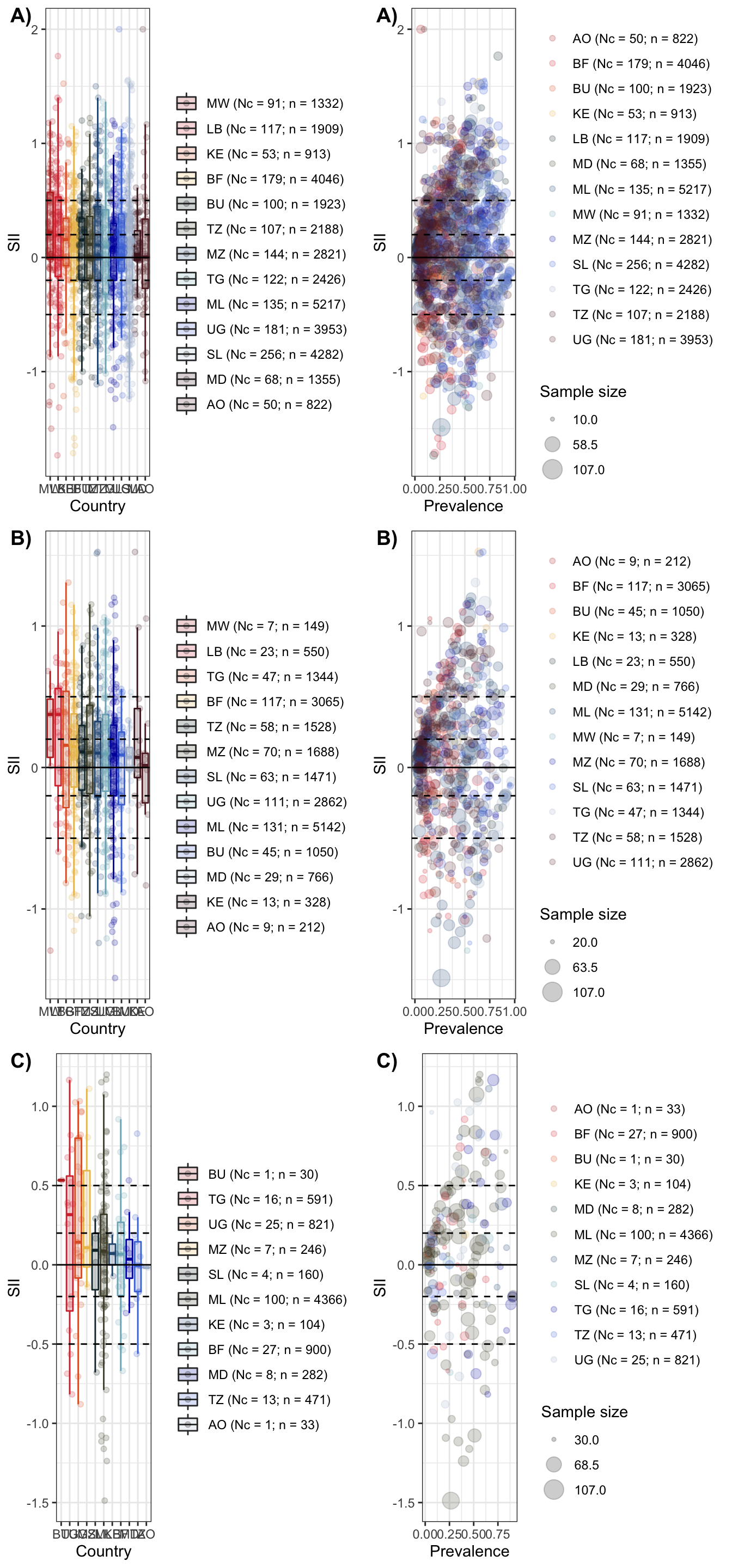
4.4.2 Maps SII - Education
Figure 01_b
Supplementary Figure 07_b
# library(mapview)
#
# m1 <- dat_edu_map %>%
#   filter(!is.na(sii)) %>%
#   mapview(zcol = "sii", legend = TRUE, layer.name = "SII (psu)")
#
# m2 <- dat_edu_adm %>%
#   mapview(zcol = "sii", legend = TRUE, layer.name = "SII (Adm)")
#
# m1 + m2

library(colorspace)

(sf7_b <- ggplot() +
  geom_sf(data = sPDF, fill = "grey") +
  geom_sf(data = dat_edu_map %>%
            filter(!is.na(sii)),
          aes(col = sii), size = .5, alpha =.6) +
  geom_sf(data = sPDF, fill = NA) +
  scale_color_continuous_diverging(palette = "Tropic") +
  labs(tag = "B)", color = "SII") +
  theme_bw())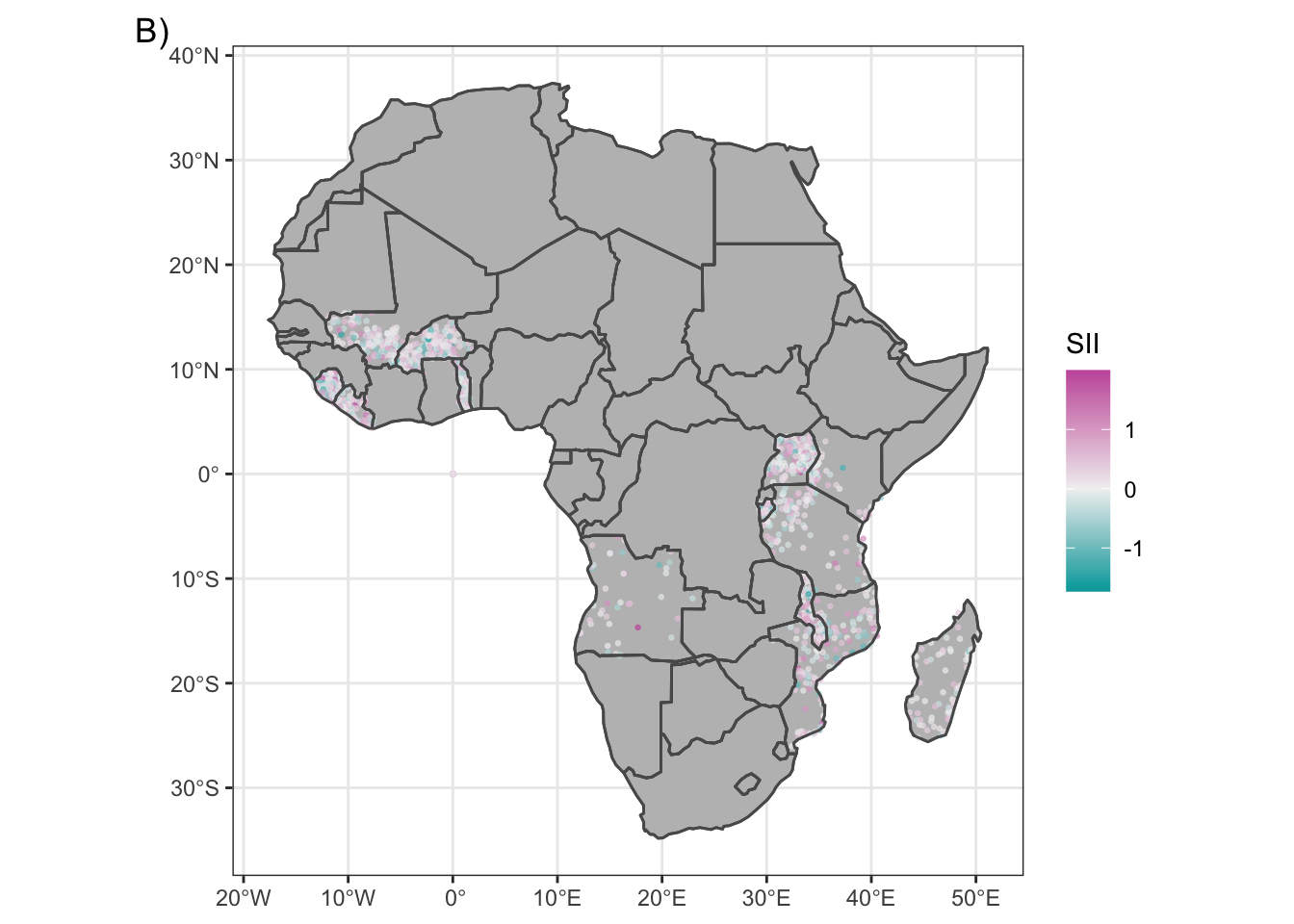
(f1_b <- ggplot() +
  geom_sf(data = sPDF, fill = "grey") +
  geom_sf(data = dat_edu_adm, aes(fill = sii),
          size = 0) +
  geom_sf(data = sPDF, fill = NA) +
  scale_fill_continuous_diverging(palette = "Tropic") +
  labs(tag = "B)", fill = "SII") +
  theme_bw())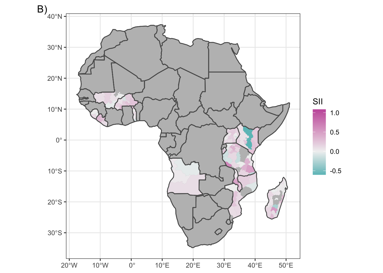
4.5 RII - Education
4.5.1 Plots RII - Education
Supplementary Figure 05
library(cowplot)
rii_box_10 <- dat_edu_map %>% filter(sample.size>=10) %>% filter(rii>0) %>% ci_box(var = rii, y_lab = "log RII", r = T) + scale_y_log10()
rii_box_20 <- dat_edu_map %>% filter(sample.size>=20) %>% filter(rii>0) %>% ci_box(var = rii, y_lab = "log RII", r = T) + scale_y_log10()
rii_box_30 <- dat_edu_map %>% filter(sample.size>=30) %>% filter(rii>0) %>% ci_box(var = rii, y_lab = "log RII", r = T) + scale_y_log10()

rii_box <- plot_grid(rii_box_10, rii_box_20, rii_box_30, labels = c("A)", "B)", "C)"), ncol = 1)

rii_prev_10 <- dat_edu_map %>% filter(sample.size>=10) %>% filter(rii>0) %>% ci_prev(var = rii, y_lab = "log RII", r = T) + scale_y_log10()
rii_prev_20 <- dat_edu_map %>% filter(sample.size>=20) %>% filter(rii>0) %>% ci_prev(var = rii, y_lab = "log RII", r = T) + scale_y_log10()
rii_prev_30 <- dat_edu_map %>% filter(sample.size>=30) %>% filter(rii>0) %>% ci_prev(var = rii, y_lab = "log RII", r = T) + scale_y_log10()

rii_prev <- plot_grid(rii_prev_10, rii_prev_20, rii_prev_30, labels = c("A)", "B)", "C)"), ncol = 1)

(sf5 <- plot_grid(rii_box, rii_prev, ncol = 2))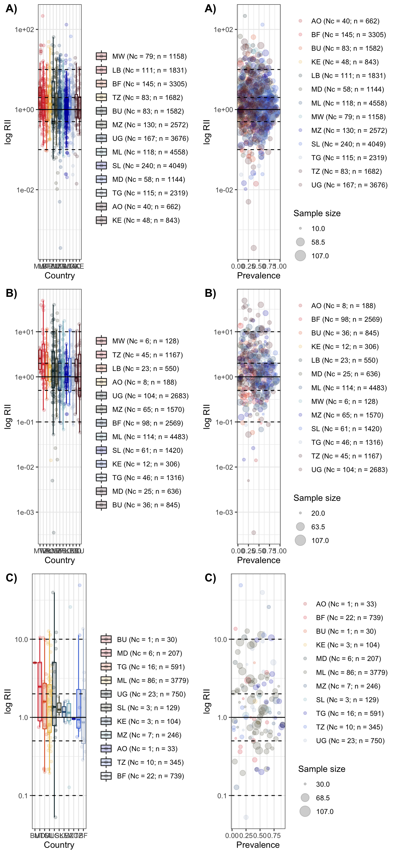
4.5.2 Maps RII - Education
Figure 02_b
Supplementary Figure 08_b
# library(mapview)
#
# m1 <- dat_edu_map %>%
#   filter(!is.na(rii)) %>%
#   mutate(log_rii = log(rii)) %>%
#   filter(log_rii != Inf & log_rii != -Inf) %>%
#   mapview(zcol = "log_rii", legend = TRUE, layer.name = "log RII (psu)")
#
# m2 <- dat_edu_adm %>%
#   filter(!is.na(rii)) %>%
#   mutate(log_rii = log(rii)) %>%
#   filter(log_rii != Inf & log_rii != -Inf) %>%
#   mapview(zcol = "log_rii", legend = TRUE, layer.name = "log RII (Adm)")
#
# m1 + m2

library(colorspace)

(sf8_b <- ggplot() +
  geom_sf(data = sPDF, fill = "grey") +
  geom_sf(data = dat_edu_map %>%
            filter(!is.na(rii)) %>%
            mutate(log_rii = log(rii)) %>%
            filter(log_rii != Inf & log_rii != -Inf),
          aes(col = log_rii), size = .5, alpha =.6) +
  geom_sf(data = sPDF, fill = NA) +
  scale_color_continuous_diverging(palette = "Tropic") +
  labs(tag = "A)", color = "log RII") +
  theme_bw())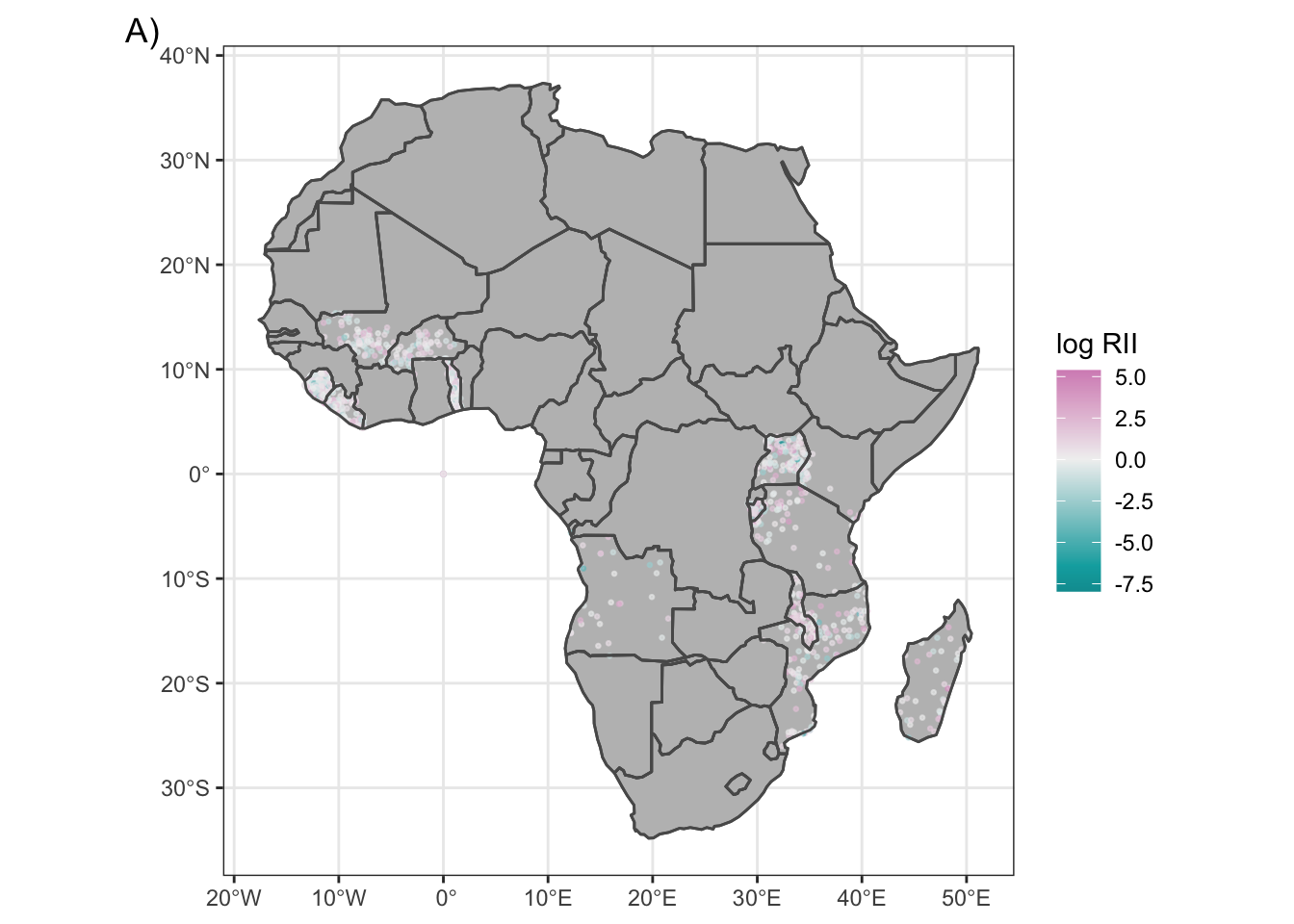
(f2_b <- ggplot() +
  geom_sf(data = sPDF, fill = "grey") +
  geom_sf(data = dat_edu_adm %>%
            filter(!is.na(rii)) %>%
            mutate(log_rii = log(rii)) %>%
            filter(log_rii != Inf & log_rii != -Inf),
          aes(fill = log_rii),
          size = 0) +
  geom_sf(data = sPDF, fill = NA) +
  scale_fill_continuous_diverging(palette = "Tropic") +
  labs(tag = "A)", fill = "log RII") +
  theme_bw())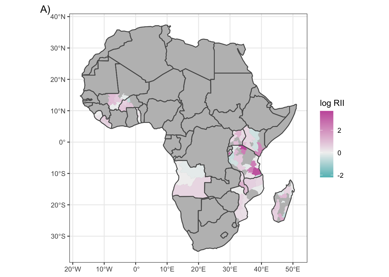
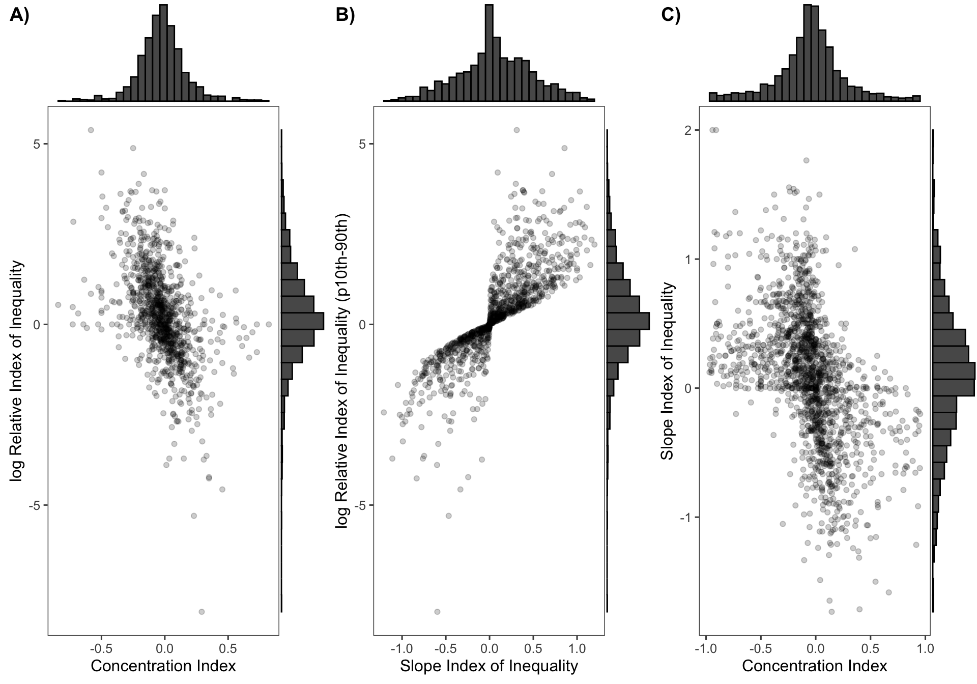
4.6 Summary -Education
Supplementary Figure 06_b
library(cowplot)
a <- dat_edu_map %>%
  filter(!is.na(rii)) %>%
  mutate(log_rii = log(rii)) %>%
  filter(log_rii != Inf & log_rii != -Inf) %>%
  bi_hist_ineq(var_x = ci_val, var_y = log_rii, lab_x = "Concentration Index", lab_y = "log Relative Index of Inequality")

b <- dat_edu_map %>%
  filter(!is.na(rii)) %>%
  mutate(log_rii = log(rii)) %>%
  filter(log_rii != Inf & log_rii != -Inf) %>%
  bi_hist_ineq(var_x = sii, var_y = log_rii, lab_x = "Slope Index of Inequality", lab_y = "log Relative Index of Inequality (p10th-90th)")

c <- dat_edu_map %>%
  bi_hist_ineq(var_x = ci_val, var_y = sii, lab_x = "Concentration Index", lab_y = "Slope Index of Inequality")

(indexes <- plot_grid(a,b,c, labels = c("A)", "B)","C)"), nrow = 1))