Chapter 2 IPTW 3
Non-linear Age
2.1 Data
rm(list = ls())
library(tidyverse)
library(kableExtra)
library(jtools)
library(sf)
load("./_data/rscd_jr.RData")

dat <- d2 %>%
  dplyr::select(id_house, comm, id_study:viaje_ult_mes,SEROPOSITIVE, main_act_ec, area) %>%
  st_set_geometry(NULL) %>%
  mutate(viaje_ult_mes = ifelse(viaje_ult_mes=="9999", NA, viaje_ult_mes),
         viaje_ult_mes = factor(ifelse(viaje_ult_mes=="2", "1_yes", "0_no")),
         SEROPOSITIVE = ifelse(SEROPOSITIVE=="Positive",1,0),
         work_out = factor(ifelse(as.numeric(main_act_ec)>0 & as.numeric(main_act_ec)<6, "outside", "inside"))) %>% filter(complete.cases(.))

dat_gf <- dat %>%
  dplyr::select(viaje_ult_mes, work_out, edad, SEROPOSITIVE, nm_sex, comm, area) %>%
  mutate(id = seq(1:n()),
         time = 0,
         viaje_ult_mes = as.integer(as.numeric(viaje_ult_mes)-1),
         work_out = as.numeric(work_out)-1,
         sex_male = as.numeric(nm_sex)-1,
         SEROPOSITIVE = as.integer(SEROPOSITIVE),
         edad = as.numeric(edad),
         edad = edad*edad
         ) %>%
  filter(complete.cases(.)) %>%
  as.data.frame()
2.2 The product method
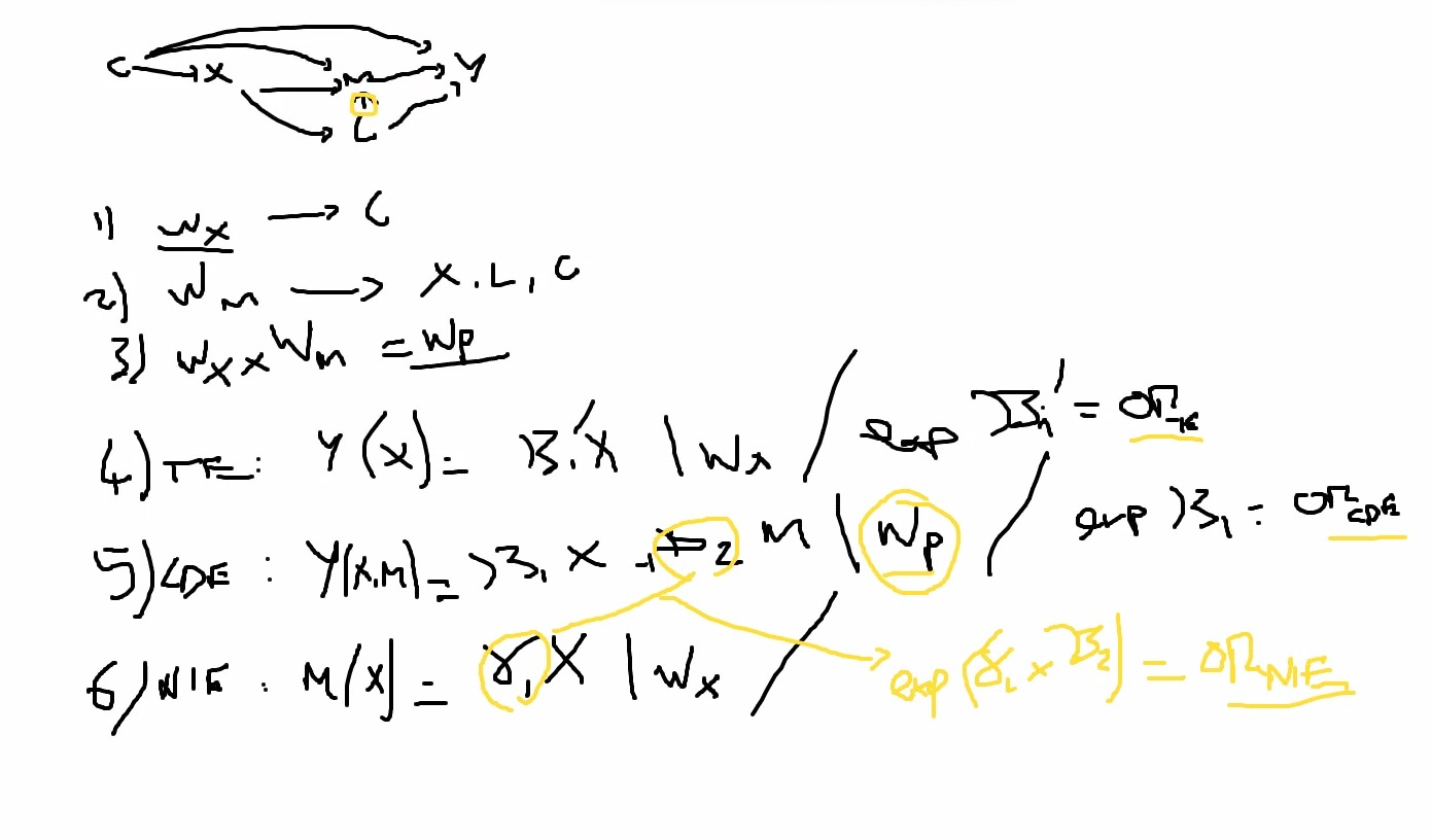
2.3 Weights
#C = edad
#X = sex_male
#M = viaje_ult_mes
#L = work_out
#Y = SEROPOSITIVE

#p1 <- glm(sex_male ~ ... , data = dat_gf, family = "binomial")
dat_gf <- dat_gf %>%
  mutate(wx = 1) #%>%
  # mutate(ps1 = predict(p1, type = "response"),
  #        wx = ifelse(sex_male==1, 1/ps1, 1/(1-ps1)))

p2 <- glm(viaje_ult_mes ~ (sex_male + work_out + edad)^2, data = dat_gf, family = "binomial")
dat_gf <- dat_gf %>%
  mutate(ps2 = predict(p2, type = "response"),
         wm = ifelse(viaje_ult_mes==1, 1/ps2, 1/(1-ps2)),
         wp = wm*wx)

dat_gf %>%
  ggplot(aes(x=wp, fill= factor(viaje_ult_mes))) +
  geom_density(alpha=.5) +
  scale_x_continuous(trans = "log10") +
  theme_nice() +
  theme(legend.position = "top")
2.4 Mediation
# Total Effect
te <- glm(SEROPOSITIVE ~ sex_male + comm, data = dat_gf, weights = wx, family = "binomial")
(te.t <- summ(te, confint = T))| Observations | 1773 |
| Dependent variable | SEROPOSITIVE |
| Type | Generalized linear model |
| Family | binomial |
| Link | logit |
| 𝛘²(10) | 186.51 |
| Pseudo-R² (Cragg-Uhler) | 0.13 |
| Pseudo-R² (McFadden) | 0.08 |
| AIC | 2292.14 |
| BIC | 2352.43 |
| Est. | 2.5% | 97.5% | z val. | p | |
|---|---|---|---|---|---|
| (Intercept) | -0.80 | -1.07 | -0.52 | -5.63 | 0.00 |
| sex_male | 0.30 | 0.11 | 0.50 | 3.01 | 0.00 |
| comm502 | 0.74 | 0.38 | 1.09 | 4.07 | 0.00 |
| comm503 | -0.19 | -0.56 | 0.19 | -0.97 | 0.33 |
| comm901 | 2.60 | 1.70 | 3.49 | 5.68 | 0.00 |
| comm902 | 1.75 | 1.31 | 2.18 | 7.94 | 0.00 |
| comm903 | 1.36 | 0.74 | 1.98 | 4.28 | 0.00 |
| comm904 | 0.52 | 0.16 | 0.87 | 2.85 | 0.00 |
| comm905 | -0.17 | -0.67 | 0.34 | -0.65 | 0.52 |
| comm906 | 0.64 | 0.23 | 1.04 | 3.06 | 0.00 |
| comm907 | 1.13 | 0.74 | 1.53 | 5.61 | 0.00 |
| Standard errors: MLE |
(te.e <- te.t$coeftable[2,1])## [1] 0.3031542# Controlled Direct Effect
cde <- glm(SEROPOSITIVE ~ sex_male + viaje_ult_mes + comm, data = dat_gf, weights = wp, family = "binomial")
(cde.t <- summ(cde, confint = T))| Observations | 1773 |
| Dependent variable | SEROPOSITIVE |
| Type | Generalized linear model |
| Family | binomial |
| Link | logit |
| 𝛘²(11) | 340.75 |
| Pseudo-R² (Cragg-Uhler) | 0.18 |
| Pseudo-R² (McFadden) | 0.07 |
| AIC | 4534.01 |
| BIC | 4599.78 |
| Est. | 2.5% | 97.5% | z val. | p | |
|---|---|---|---|---|---|
| (Intercept) | -0.79 | -1.03 | -0.56 | -6.62 | 0.00 |
| sex_male | 0.16 | 0.02 | 0.30 | 2.21 | 0.03 |
| viaje_ult_mes | 0.02 | -0.14 | 0.18 | 0.22 | 0.83 |
| comm502 | 0.83 | 0.52 | 1.13 | 5.28 | 0.00 |
| comm503 | -0.12 | -0.45 | 0.21 | -0.70 | 0.48 |
| comm901 | 2.39 | 1.89 | 2.89 | 9.36 | 0.00 |
| comm902 | 1.66 | 1.35 | 1.97 | 10.65 | 0.00 |
| comm903 | 1.61 | 1.20 | 2.03 | 7.55 | 0.00 |
| comm904 | 0.62 | 0.34 | 0.91 | 4.34 | 0.00 |
| comm905 | 0.06 | -0.30 | 0.42 | 0.34 | 0.73 |
| comm906 | 0.67 | 0.37 | 0.98 | 4.40 | 0.00 |
| comm907 | 1.02 | 0.72 | 1.32 | 6.69 | 0.00 |
| Standard errors: MLE |
(cde.e <- cde.t$coeftable[2,1])## [1] 0.1569569(b2 <- cde.t$coeftable[3,1])## [1] 0.01838016# Natual Indirect Effect
nie <- glm(viaje_ult_mes ~ sex_male + comm, data = dat_gf, weights = wx, family = "binomial")
(nie.t <- summ(nie, confint = T))| Observations | 1773 |
| Dependent variable | viaje_ult_mes |
| Type | Generalized linear model |
| Family | binomial |
| Link | logit |
| 𝛘²(10) | 392.14 |
| Pseudo-R² (Cragg-Uhler) | 0.32 |
| Pseudo-R² (McFadden) | 0.22 |
| AIC | 1377.34 |
| BIC | 1437.62 |
| Est. | 2.5% | 97.5% | z val. | p | |
|---|---|---|---|---|---|
| (Intercept) | -3.06 | -3.66 | -2.47 | -10.13 | 0.00 |
| sex_male | 0.17 | -0.09 | 0.43 | 1.27 | 0.21 |
| comm502 | -0.99 | -2.05 | 0.07 | -1.84 | 0.07 |
| comm503 | -15.57 | -804.88 | 773.74 | -0.04 | 0.97 |
| comm901 | 2.95 | 2.13 | 3.76 | 7.09 | 0.00 |
| comm902 | 2.65 | 2.00 | 3.31 | 7.97 | 0.00 |
| comm903 | 2.64 | 1.85 | 3.43 | 6.56 | 0.00 |
| comm904 | 1.90 | 1.26 | 2.54 | 5.81 | 0.00 |
| comm905 | 2.02 | 1.29 | 2.75 | 5.42 | 0.00 |
| comm906 | 2.82 | 2.16 | 3.47 | 8.38 | 0.00 |
| comm907 | 1.68 | 1.01 | 2.36 | 4.87 | 0.00 |
| Standard errors: MLE |
(a1 <- nie.t$coeftable[2,1])## [1] 0.169106(nie.e <- a1*b2) ## [1] 0.003108195# TE
cde.e + nie.e## [1] 0.1600651te.e## [1] 0.3031542# PROPORTION MEDIATED
(exp(cde.e)*(exp(nie.e)-1))/((exp(cde.e)*exp(nie.e))-1)## [1] 0.020981232.5 BOOTSTRAP NIE
library(boot)

i = c("SEROPOSITIVE","sex_male","viaje_ult_mes","area")
fc <- function(tab, i){
  d2 <- tab[i,]
  #CDE
  mod2 <- glm(SEROPOSITIVE ~ sex_male + viaje_ult_mes + area, data = d2, weights = wp, family = "binomial")
  #NIE
  medmod <- glm(viaje_ult_mes ~ sex_male + area, data = d2, weights = wx, family = "binomial")
  out <- coef(summary(medmod))[2,1]*coef(summary(mod2))[3,1]
  return(out)
}

bootm=boot(dat_gf,fc,R=5)
mean <- bootm$t0
ci <- boot.ci(boot.out = bootm, type = c("basic"))$basic[4:5]

print(c(mean=mean, lower.limit=ci[1], upper.limit=ci[2]))
## mean lower.limit upper.limit
## 0.02371722 -0.01615326 0.08430095print(exp(c(mean=mean, lower.limit=ci[1], upper.limit=ci[2])))## mean lower.limit upper.limit
## 1.0240007 0.9839765 1.08795632.6 MEDIATION PACKAGE
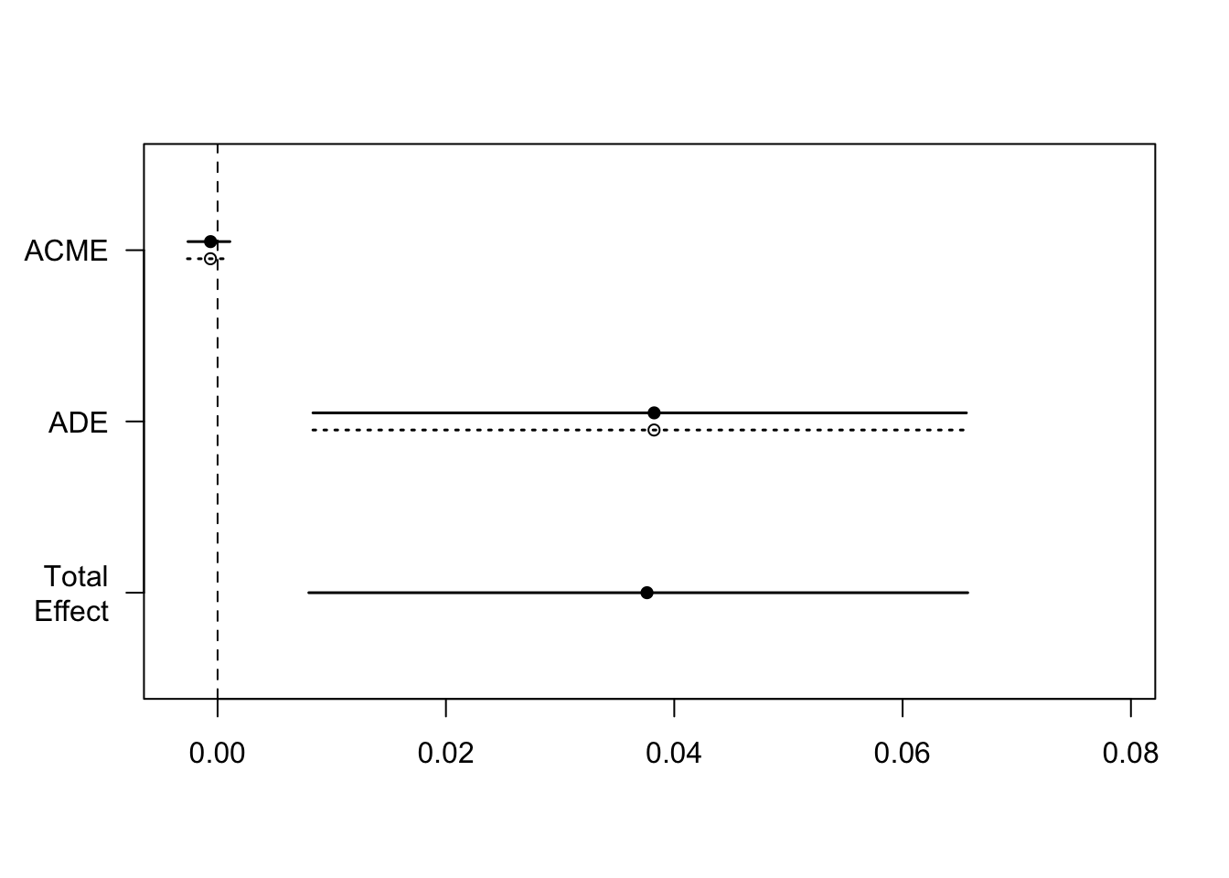
- average causal mediation effects (ACME)
- average direct effects (ADE)
library(mediation)
#Error in mediate(med.fit, out.fit, treat = "sex_male", mediator = "viaje_ult_mes", : weights on outcome and mediator models not identical
med.fit <- glm(viaje_ult_mes ~ sex_male + area, data = dat_gf, weights = wp, family = "binomial")
out.fit <- glm(SEROPOSITIVE ~ sex_male + viaje_ult_mes + area, data = dat_gf, weights = wp, family = "binomial")
med.out <- mediate(med.fit, out.fit, treat = "sex_male", mediator = "viaje_ult_mes", sims = 100)
summary(med.out)
##
## Causal Mediation Analysis
##
## Quasi-Bayesian Confidence Intervals
##
## Estimate 95% CI Lower 95% CI Upper p-value
## ACME (control) -0.000627 -0.002641 0.00 0.42
## ACME (treated) -0.000617 -0.002596 0.00 0.42
## ADE (control) 0.038229 0.008352 0.07 0.02 *
## ADE (treated) 0.038238 0.008353 0.07 0.02 *
## Total Effect 0.037611 0.007988 0.07 0.02 *
## Prop. Mediated (control) -0.017456 -0.102073 0.04 0.44
## Prop. Mediated (treated) -0.017102 -0.100996 0.04 0.44
## ACME (average) -0.000622 -0.002618 0.00 0.42
## ADE (average) 0.038233 0.008353 0.07 0.02 *
## Prop. Mediated (average) -0.017279 -0.101535 0.04 0.44
## ---
## Signif. codes: 0 '***' 0.001 '**' 0.01 '*' 0.05 '.' 0.1 ' ' 1
##
## Sample Size Used: 1773
##
##
## Simulations: 100plot(med.out)