Chapter 4 Working with data
Now we can take a first dive into data wrangling. First of all, we need to read in the data into our R session. I will talk about that maybe longer than I should. Thereafter, we need to make sure that the data is in the right format. You probably have not really thought about how a data set is supposed to look like. The concept of tidy data provides you an idea for this.
4.1 Reading in data sets
First, the readr package (Hester et al. 2018) will be introduced. It can be used for the import of the majority of files you will ever want to import and export. If the files become larger, vroom (Hester et al. 2020) is a viable alternative. Beyond that, there exist some more packages for other types such as Excel or Stata files. I will provide you with a basic tutorial on how to deal with them, too.
Some notes on the notation: "file.csv" relates to the file you want to read in – please note that it needs to be provided as a character vector, tibble to the Tibble you want to write.
4.1.1 The working directory in R
As mentioned when introducing RStudio Projects, there are two kinds of file paths you can provide R with: absolute and relative paths.
The absolute path for this script on my machine looks like this: “/Users/felixlennert/Documents/phd/teaching/introduction-to-r/03-tidying.Rmd.”
If you are on a Windows machine and copy file paths: R uses the file path separator \ as a so-called escape character – hence, it does not recognize it as a file path separator. You can address this problem by either using double back-slashes \\ or using a normal slash, /, instead.
There is always a working directory you are in. You can obtain your working directory using getwd(). Relative paths then just build upon it. If you want to change your working directory, use setwd().
Please note that I included the former two paragraphs just for the record. You should never use absolute paths, except for if you are planning to keep the same machine for the rest of your life and never change any of your file structure. You are not. Hence, please use RStudio Projects.4
If you are using RStudio Projects, your working directory defaults to the folder your .Rproj file is stored in.
If you are working in RMarkdown, the working directory is where your RMarkdown document is stored in.
4.1.2 readr’s general functions…
In general, importing data with readr is pretty hassle-free: the hardest thing about it is calling the right function. It usually takes care of the rest itself, parsing columns properly, etc. However, sometimes you need to specify additional arguments.
The following unordered list shows the most common read_*() functions. Usually, you can simply provide them a file path and they load in the data and return a Tibble. If your data is in a compressed file with the extension .gz, .bz2, .xz, or .zip, readr will automatically uncompress it. If the file is stored online, you can provide a URL starting with http://, https://, ftp://, or ftps://. readr will automatically take care of the download process.
read_csv("file.csv")reads comma delimited files
read_csv2("file.csv")reads semi-colon delimited files and treats commas as decimal separator
read_delim("file.txt", delim = "|")reads files which are delimited by whatever delimiter you specify (|in this case)
read_fwf("file.fwf", col_positions = c(1, 3, 5))reads fixed width files. Here, some sort of data on the columns must be provided, e.g., their positions in the file
- If the values are separated by white space, you can also use
read_tsv("file.tsv")orread_table("file.tsv")
4.1.3 …and their additional arguments
Also, all these functions share certain arguments which just need to be included in the call. In the following, I will enumerate the most useful ones.
- If your file does not have a header (most of the time, column names), provide
col_names = FALSE. The resulting Tibble will haveX1 … Xnas column names
- If your file does not have column names, but you want the resulting Tibble to have some, you can specify them with
col_names = c("a", "b", "c"). It takes a character vector.
- If there are rows you do not want to be considered, you can use
skip =. For instance,read_csv("file.csv", skip = 6)reads everything but the first six data rows (the very first row is not taken into consideration as well)
- Sometimes the original creator of your data set might go across missing values differently than you would want it to.
na =can be used to specify which values shall be considered missing. If your missings are coded as 99 and 999, for instance, you can address that in the read-in process already by usingread_csv("file.csv", na = c("99", "999")). Please note that it takes a character vector as argument
- In some data sets, the first rows consists of comments that start with particular signs or special characters. Using
comment =allows you to skip these lines. For instance,read_csv("file.csv", comment = "#")drops all the rows that begin with a hash.
4.1.4 Column types
As you have already learned in the script before, a Tibble consists of multiple vectors of the same length. The vectors can be of different types. When you read in data using readr, it will print out the column types it has guessed. When you read in data, you must ascribe it to an object in your environment. The following code reads in a .csv file with data on the 100 most-played songs on Spotify in 2018 and stores it in the object spotify_top100_2018.
library(tidyverse)
# library(readr) --> no need to load readr, it's part of the core tidyverse
spotify_top100_2018 <- read_csv("data/spotify2018.csv")
## Rows: 100 Columns: 16## ── Column specification ────────────────────────────────────────────────────────
## Delimiter: ","
## chr (3): id, name, artists
## dbl (13): danceability, energy, key, loudness, mode, speechiness, acousticne...##
## ℹ Use `spec()` to retrieve the full column specification for this data.
## ℹ Specify the column types or set `show_col_types = FALSE` to quiet this message.If your data is well-behaved, R will guess the vector types correctly and everything will run smoothly. However, sooner or later you will stumble across a data set which is not well-behaved. This is where knowing how to fine-tune your parsing process up-front will eventually save you a lot of head scratching.
But how does parsing actually look like. Well, readr’s parsing functions take a character vector and return a more specialized vector.
parse_double(c("1", "2", "3"))## [1] 1 2 3So far so good. What readr does when it reads in your data sets is that it tries to guess the correct data type. This can be emulated using guess_parser() and parse_guess(). Both functions take a character vector as input. The former one returns the guessed type, the latter returns a vector which is parsed to the type it has guessed.
guess_parser("2009-04-23")## [1] "date"str(parse_guess("2009-04-23"))## Date[1:1], format: "2009-04-23"The heuristic it uses is fairly simple yet robust. However, there are common cases when you might run into problems with different data types. In the following, I will show you the two most common ones. The first one regards numeric data, the second one data on date and time.
4.1.4.1 Numbers
Parsing numbers should be straight-forward, right, so what could possibly go wrong?
Well…
- Decimal points
- Special characters ($, %, §, €)
- So-called grouping characters such as 1,000,000 (USA) or 1.000.000 (Germany) or 1’000’000 (Switzerland)
The problem with decimal points (– and commas) can be addressed by specifying a locale. Compare:
parse_double("1,3")## Warning: 1 parsing failure.
## row col expected actual
## 1 -- no trailing characters 1,3## [1] NA
## attr(,"problems")
## # A tibble: 1 × 4
## row col expected actual
## <int> <int> <chr> <chr>
## 1 1 NA no trailing characters 1,3parse_double("1,3", locale = locale(decimal_mark = ","))## [1] 1.3The special character problem can be addressed using parse_number instead of parse_double: it will ignore the special characters.
parse_number("1.5€")## [1] 1.5The last problem can be addressed using another locale.
parse_number("1.300.000", locale = locale(grouping_mark = "."))## [1] 13000004.1.4.2 Date and time
Date vectors in R are numeric vectors indicating how many days have passed since 1970. Date-Time vectors indicate the seconds since 1970-01-01 00:00:00. Time vectors indicate the number of seconds since midnight.
The parse_*() functions expect the vectors to be in a certain format:
parse_datetime()expects the input to follow the ISO8601 standard. The times components must be ordered from biggest to smallest: year, month, day, hour, minute, second.
parse_datetime("2000-02-29T2000")## [1] "2000-02-29 20:00:00 UTC"parse_date()wants a four digit year, two digit month, and two digit day. They can be separated by either “-” or “/.”
parse_date("2000-02-29")## [1] "2000-02-29"parse_date("2000/02/29")## [1] "2000-02-29"Do you wonder why I chose 2000-02-29? It’s R’s birthday…
parse_time()needs at least hours and minutes, seconds are optional. They need to be separated by colons. There is no proper built-in class for time data in Base R. Hence, I will use thehmspackage here.
library(hms)##
## Attaching package: 'hms'## The following object is masked from 'package:lubridate':
##
## hmsparse_time("20:15:00")## 20:15:00parse_time("20:15") # both works## 20:15:00When it comes to dates, you can also build your own format. Just mash together the following pieces:
- Year:
%Y– year in 4 digits;%y– year in two digits following this rule: 00–69 = 2000–2069, 70–99 = 1970–1999
- Month:
%m– two digits;%b– abbreviated name (e.g., “Nov”);%B– full name (e.g., “November”)
- Day:
%d– two digits
- Time:
%H– hour, 0–23;%h– hour, 1–12, must come together with%p– a.m./p.m. indicator;%M– minutes;%S– integer seconds;%Ztime zone –America/Chicagofor instance
- Non-digits:
%.skips one non-digit character;%*skips any number of non-digits
You might see that there can emerge problems with this. You might, for example, have something like this:
example_date <- "29. Februar 2000"So how can you parse this date with a German month name? Again, you can use locale =.
date_names_langs() # what could be the proper abbreviation?## [1] "af" "agq" "ak" "am" "ar" "as" "asa" "az" "bas" "be" "bem" "bez"
## [13] "bg" "bm" "bn" "bo" "br" "brx" "bs" "ca" "cgg" "chr" "cs" "cy"
## [25] "da" "dav" "de" "dje" "dsb" "dua" "dyo" "dz" "ebu" "ee" "el" "en"
## [37] "eo" "es" "et" "eu" "ewo" "fa" "ff" "fi" "fil" "fo" "fr" "fur"
## [49] "fy" "ga" "gd" "gl" "gsw" "gu" "guz" "gv" "ha" "haw" "he" "hi"
## [61] "hr" "hsb" "hu" "hy" "id" "ig" "ii" "is" "it" "ja" "jgo" "jmc"
## [73] "ka" "kab" "kam" "kde" "kea" "khq" "ki" "kk" "kkj" "kl" "kln" "km"
## [85] "kn" "ko" "kok" "ks" "ksb" "ksf" "ksh" "kw" "ky" "lag" "lb" "lg"
## [97] "lkt" "ln" "lo" "lt" "lu" "luo" "luy" "lv" "mas" "mer" "mfe" "mg"
## [109] "mgh" "mgo" "mk" "ml" "mn" "mr" "ms" "mt" "mua" "my" "naq" "nb"
## [121] "nd" "ne" "nl" "nmg" "nn" "nnh" "nus" "nyn" "om" "or" "os" "pa"
## [133] "pl" "ps" "pt" "qu" "rm" "rn" "ro" "rof" "ru" "rw" "rwk" "sah"
## [145] "saq" "sbp" "se" "seh" "ses" "sg" "shi" "si" "sk" "sl" "smn" "sn"
## [157] "so" "sq" "sr" "sv" "sw" "ta" "te" "teo" "th" "ti" "to" "tr"
## [169] "twq" "tzm" "ug" "uk" "ur" "uz" "vai" "vi" "vun" "wae" "xog" "yav"
## [181] "yi" "yo" "zgh" "zh" "zu"parse_date(example_date, format = "%d%. %B %Y", locale = locale(date_names = "de"))## [1] "2000-02-29"Now you know how to parse number and date vectors yourself. This is nice, but normally you do not want to read in data, put it into character vectors and then parse it to the right data format. You want to read in a data set and get a Tibble whose columns consist of data which have been parsed to the right type already.
4.1.4.3 Parsing entire files
As mentioned earlier, the read_* functions guess the columns format. I emulated this using the guess_parser() function.
If you want to specify the column types yourself, you can use the col_types = argument:
challenge_w_date <- read_csv(readr_example("challenge.csv"),
                             col_types = cols(
                               x = col_number(),
                               y = col_date()
                             ))
In general, every parse_* function has its col_* counterpart.
4.2 Alternative ways to read in and write data
There do also other packages exist for different data types. I will explain the ones which might be of particular use for you and their main-functions only briefly.
4.2.1 haven
You can use haven (Wickham and Miller 2020) for reading and writing SAS (suffixes .sas7bdat, .sas7bcat, and .xpt), SPSS (suffixes .sav and .por), and STATA (suffix .dta) files.
The functions then are:
read_sas("file.sas7bdate")andwrite_sas(tibble, "file.sas7bdat")for both.sas7bdatand.sas7bcatfiles.read_xpt("file.xpt")reads.xptfiles
read_sav("file.sav")andread_por("file.por")for.savand.porfiles.write_sav(tibble, "file.sav"writes a the Tibbletibbleto the filefile.sav
read_dta("file.dta")andwrite_dta(tibble, "file.dta")read and write.dtafiles
The additional arguments can be found in the vignette.
4.2.2 readxl
readxl (Wickham, Bryan, et al. 2019) can be used to read Excel files. read_excel("file.xls") works for both .xls and .xlsx files alike. It guesses the data type from the suffix. Excel files often consist of multiple sheets. excel_sheets("file.xlsx") returns the name of the singular sheets. When dealing with an Excel file that contains multiple sheets, you need to specify the sheet you are after in the read_excel() function: read_excel("file.xlsx", sheet = "sheet_1"). Please note that it only takes one sheet at a time.
More on the readxl package can be found here.
4.2.3 vroom
vroom has been introduced recently. It claims to be able to read in delimited files with up to 1.4 GB/s. Regarding its arguments, vroom works in the same way as the read_*() functions from the readr package. I would recommend you to use vroom as soon as your data set’s size exceeds ~100 MB.
4.3 Write data
4.3.1 write_csv()
Writing data is fairly straight-forward. Most of the times, you will work with plain Tibbles which consist of different kinds of vectors except for lists. If you want to store them, I recommend you to simply use write_csv(tibble, path = "file.csv"). If you plan on working on the .csv file in Excel, use write_excel_csv(tibble, path = "file.csv")
4.3.2 write_rds()
Sometimes, however, it might be impossible to create a .csv file of your data – e.g., if you want to store a list. This is what you can use write_rds(r_specific_object, path = "file.rds") for.
4.3.3 save()
Akin to .rds files are .RData files. They can contain multiple objects and be written using save(r_specific_object_1, r_specific_object_2, r_specific_object_n, file = "file.RData"). You can save your entire work space as well by calling save.image(file = "file.RData").
4.3.4 Further readings
- Information on working directories
- Websites of the singular packages: readr, haven, readxl, vroom
readrCheatsheet
- Chapter in R for Data Science (Wickham and Grolemund 2016) regarding data import
4.4 Tidy data
Before you learn how to tidy and wrangle data, you need to know how you want your data set to actually look like, i.e., what the desired outcome of the entire process of tidying your data set is. The tidyverse is a collection of packages which share an underlying philosophy: they are tidy. This means, that they (preferably) take tidy data as inputs and output tidy data. In the following, I will, first, introduce you to the concept of tidy data as developed by Hadley Wickham (Wickham 2014). Second, tidyr is introduced (Wickham 2020b). Its goal is to provide you with functions that facilitate tidying data sets. Beyond, I will provide you some examples of how to create tibbles using functions from the tibble package (Müller, Wickham, and François 2020). Moreover, the pipe from the magrittr package is introduced.
Please note that tidying and cleaning data are not equivalent: I refer to tidying data as to bringing data in a tidy format. Cleaning data, however, can encompass way more than this: parsing columns in the right format (using readr, for instance), imputation of missing values, address the problem of typos, etc.
4.4.1 In theory
Data sets can be structured in many ways. To make them tidy, they must be organized in the following way (this is taken from the R for Data Science book (Wickham and Grolemund 2016)):
- Each variable must have its own column.
- Each observation must have its own row.
- Each value must have its own cell.
They can even be boiled further down:
- Put each data set in a tibble.
- Put each variable in a column.
This can also be visually depicted:
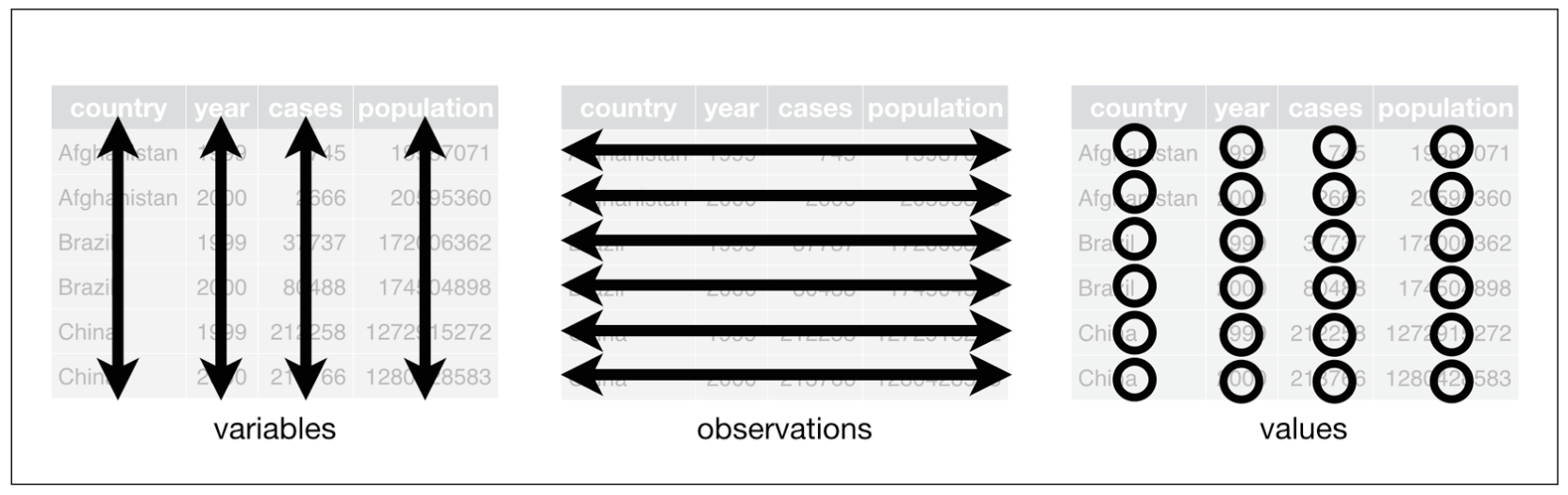
The three rules that make a dataset tidy (taken from Wickham and Grolemund 2016: 149)
This way of storing data has two big advantages:
- you can easily access, and hence manipulate, variables as vectors
- if you perform vectorized operations on the tibble, cases are preserved.
4.4.2 In practice
So what are the most common problems with data sets? The following list is taken from the tidyr vignette5:
- Column headers are values, not variable names.
- Variables are stored in both rows and columns.
- Multiple variables are stored in one column.
- Multiple types of observational units are stored in the same table.
- A single observational unit is stored in multiple tables.
I will go across the former three types of problems, because the latter two require some more advanced data wrangling techniques you haven’t learned yet (i.e., functions from the dplyr package: select(), mutate(), left_join(), among others).
In the following, I will provide you with examples on how this might look like and how you can address the respective problem using functions from the tidyr package. This will serve as an introduction to the two most important functions of the tidyr package: pivot_longer() and its counterpart pivot_wider(). Beyond that, separate() will be introduced as well. At the beginning of every part, I will build the tibble using functions from the tibble package. This should suffice as a quick refresher for and introduction to creating tibbles.
tidyr has some more functions in stock. They do not necessarily relate to transforming messy data sets into tidy ones, but also serve you well for some general cleaning tasks. They will be introduced, too.
4.4.2.1 Column headers are values
A data set of this form would look like this:
tibble_value_headers <- tibble(
  manufacturer = c("Audi", "BMW", "Mercedes", "Opel", "VW"),
  `3 cyl` = sample(20, 5, replace = TRUE),
  `4 cyl` = sample(50:100, 5, replace = TRUE),
  `5 cyl` = sample(10, 5, replace = TRUE),
  `6 cyl` = sample(30:50, 5, replace = TRUE),
  `8 cyl` = sample(20:40, 5, replace = TRUE),
  `10 cyl` = sample(10, 5, replace = TRUE),
  `12 cyl` = sample(20, 5, replace = TRUE),
  `16 cyl` = rep(0, 5)
)

tibble_value_headers
## # A tibble: 5 × 9
## manufacturer `3 cyl` `4 cyl` `5 cyl` `6 cyl` `8 cyl` `10 cyl` `12 cyl`
## <chr> <int> <int> <int> <int> <int> <int> <int>
## 1 Audi 20 86 3 47 26 2 12
## 2 BMW 17 89 2 32 30 9 3
## 3 Mercedes 1 86 3 45 40 3 15
## 4 Opel 6 66 5 44 37 2 3
## 5 VW 8 85 10 50 33 8 20
## # … with 1 more variable: 16 cyl <dbl>You can create a tibble by column using the tibble function. Column names need to be specified and linked to vectors of either the same length or length one.
This data set basically consists of three variables: German car manufacturer, number of cylinders, and frequency. To make the data set tidy, it has to consist of three columns depicting the three respective variables. This operation is called pivoting the non-variable columns into two-column key-value pairs. As the data set will thereafter contain fewer columns and more rows than before, it will have become longer (or taller). Hence, the tidyr function is called pivot_longer().
ger_car_manufacturer_longer <- tibble_value_headers %>%
  pivot_longer(-manufacturer, names_to = "cylinders", values_to = "frequency")
ger_car_manufacturer_longer
## # A tibble: 40 × 3
## manufacturer cylinders frequency
## <chr> <chr> <dbl>
## 1 Audi 3 cyl 20
## 2 Audi 4 cyl 86
## 3 Audi 5 cyl 3
## 4 Audi 6 cyl 47
## 5 Audi 8 cyl 26
## 6 Audi 10 cyl 2
## 7 Audi 12 cyl 12
## 8 Audi 16 cyl 0
## 9 BMW 3 cyl 17
## 10 BMW 4 cyl 89
## # … with 30 more rowsIn the function call, you need to specify the following: if you were not to use the pipe, the first argument would be the tibble you are manipulating. Then, you look at the column you want to keep. Here, it is the car manufacturer. This means that all columns but manufacturer will be crammed into two new ones: one will contain the columns’ names, the other one their values. How are those new column supposed to be named? That can be specified in the names_to = and values_to =arguments. Please note that you need to provide them a character vector, hence, surround your parameters with quotation marks. As a rule of thumb for all tidyverse packages: If it is a new column name you provide, surround it with quotation marks. If it is one that already exists – like, here, manufacturer, then you do not need the quotation marks.
4.4.2.2 Variables in both rows and columns
You have this data set:
car_models_fuel <- tribble(~manufacturer, ~model, ~cylinders, ~fuel_consumption_type, ~fuel_consumption_per_100km,
                      "VW", "Golf", 4, "urban", 5.2,
                      "VW", "Golf", 4, "extra urban", 4.5,
                      "Opel", "Adam", 4, "urban", 4.9,
                      "Opel", "Adam", 4, "extra urban", 4.1)
car_models_fuel
## # A tibble: 4 × 5
## manufacturer model cylinders fuel_consumption_type fuel_consumption_per_100km
## <chr> <chr> <dbl> <chr> <dbl>
## 1 VW Golf 4 urban 5.2
## 2 VW Golf 4 extra urban 4.5
## 3 Opel Adam 4 urban 4.9
## 4 Opel Adam 4 extra urban 4.1It was created using the tribble function: tibbles can also be created by row. First, the column names need to be specified by putting a tilde (~) in front of them. Then, you can put in values separated by commas. Please note that the number of values needs to be a multiple of the number of columns.
In this data set, there are basically five variables: manufacturer, model, cylinders, urban fuel consumption, and extra urban fuel consumption. However, the column fuel_consumption_type does not store a variable but the names of two variables. Hence, you need to fix this to make the data set tidy. Because this encompasses reducing the number of rows, the data set becomes wider. The function to achieve this is therefore called pivot_wider() and the inverse of pivot_longer().
car_models_fuel_tidy <- car_models_fuel %>%
  pivot_wider(names_from = fuel_consumption_type, values_from = fuel_consumption_per_100km)
car_models_fuel_tidy
## # A tibble: 2 × 5
## manufacturer model cylinders urban `extra urban`
## <chr> <chr> <dbl> <dbl> <dbl>
## 1 VW Golf 4 5.2 4.5
## 2 Opel Adam 4 4.9 4.1Here, you only need to specify the columns you fetch the names and values from. As they both do already exist, you do not need to wrap them in quotation marks.
4.4.2.3 Multiple variables in one column
Now, however, there is a problem with the cylinders: their number should be depicted in a numeric vector. We could achieve this by either parsing it to a numeric vector:
parse_number(ger_car_manufacturer_longer$cylinders)## [1] 3 4 5 6 8 10 12 16 3 4 5 6 8 10 12 16 3 4 5 6 8 10 12 16 3
## [26] 4 5 6 8 10 12 16 3 4 5 6 8 10 12 16On the other hand, we can also use a handy function from tidyr called separate() and afterwards drop the unnecessary column:
ger_car_manufacturer_longer_sep_cyl <- ger_car_manufacturer_longer %>% # first, take the tibble
  separate(cylinders, into = c("cylinders", "drop_it"), sep = " ") %>% # and then split the column "cylinders" into two
  select(-drop_it) # you will learn about this in the lesson on dplyr  # and then drop one column from the tibble
If there are two (or actually more) relevant values in one column, you can simply let out the dropping process and easily split them into multiple columns. By default, the sep = argument divides the content by all non-alphanumeric characters (every character that is not a letter, number, or space) it contains.
Please note that the new column is still in character format. We can change this using as.numeric():
ger_car_manufacturer_longer_sep_cyl$cylinders <- as.numeric(ger_car_manufacturer_longer_sep_cyl$cylinders)Furthermore, you might want to sort your data in a different manner. If you want to do this by cylinders, it would look like this:
arrange(ger_car_manufacturer_longer_sep_cyl, cylinders)## # A tibble: 40 × 3
## manufacturer cylinders frequency
## <chr> <dbl> <dbl>
## 1 Audi 3 20
## 2 BMW 3 17
## 3 Mercedes 3 1
## 4 Opel 3 6
## 5 VW 3 8
## 6 Audi 4 86
## 7 BMW 4 89
## 8 Mercedes 4 86
## 9 Opel 4 66
## 10 VW 4 85
## # … with 30 more rows4.4.2.4 Insertion: the pipe
Have you noticed the %>%? That’s the pipe. It’s from the magrittr package (Bache and Wickham 2014) whose name is based on the Belgian painter who has created this masterpiece:

Just kidding:

It can be considered a conjunction in coding. Usually, you will use it when working with tibbles. What it does is pretty straight-forward: it takes what is on its left – the input – and provides it to the function on its right as the first argument. Hence, the code in the last chunk, which looks like this
arrange(ger_car_manufacturer_longer_sep_cyl, cylinders)## # A tibble: 40 × 3
## manufacturer cylinders frequency
## <chr> <dbl> <dbl>
## 1 Audi 3 20
## 2 BMW 3 17
## 3 Mercedes 3 1
## 4 Opel 3 6
## 5 VW 3 8
## 6 Audi 4 86
## 7 BMW 4 89
## 8 Mercedes 4 86
## 9 Opel 4 66
## 10 VW 4 85
## # … with 30 more rowscould have also been written like this
ger_car_manufacturer_longer_sep_cyl %>% arrange(cylinders)## # A tibble: 40 × 3
## manufacturer cylinders frequency
## <chr> <dbl> <dbl>
## 1 Audi 3 20
## 2 BMW 3 17
## 3 Mercedes 3 1
## 4 Opel 3 6
## 5 VW 3 8
## 6 Audi 4 86
## 7 BMW 4 89
## 8 Mercedes 4 86
## 9 Opel 4 66
## 10 VW 4 85
## # … with 30 more rowsbecause the tibble is the first argument in the function call.
Because magrittr really has gained traction in the R community, many functions are now optimized for being used with the pipe. However, there are still some around which are not. A function for fitting a basic linear model with one dependent and one independent variable which are both stored in a tibble looks like this: lm(formula = dv ~ iv, data = tibble). Here, the tibble is not the first argument. To be able to fit a linear model in a “pipeline,” you need to employ a little hack: you can use a dot . as a placeholder.
Let’s check out the effect the number of cylinders has on the number of models:
ger_car_manufacturer_longer_sep_cyl %>%
  lm(frequency ~ cylinders, data = .) %>%
  summary()
##
## Call:
## lm(formula = frequency ~ cylinders, data = .)
##
## Residuals:
## Min 1Q Median 3Q Max
## -38.301 -16.420 1.262 13.490 52.819
##
## Coefficients:
## Estimate Std. Error t value Pr(>|t|)
## (Intercept) 48.6623 8.3170 5.851 9.12e-07 ***
## cylinders -3.1203 0.9227 -3.382 0.00168 **
## ---
## Signif. codes: 0 '***' 0.001 '**' 0.01 '*' 0.05 '.' 0.1 ' ' 1
##
## Residual standard error: 24.24 on 38 degrees of freedom
## Multiple R-squared: 0.2313, Adjusted R-squared: 0.2111
## F-statistic: 11.44 on 1 and 38 DF, p-value: 0.00168As %>% is a bit tedious to type, there exist shortcuts: shift-ctrl-m on a Mac, shift-ctrl-m on a Windows machine.
4.4.2.5 Further functionalities
4.4.2.5.1 Splitting and merging cells
If there are multiple values in one column/cell and you want to split them and put them into two rows instead of columns, tidyr offers you the separate_rows() function.
german_cars_vec <- c(Audi = "A1, A3, A4, A5, A6, A7, A8", BMW = "1 Series, 2 Series, 3 Series, 4 Series, 5 Series, 6 Series, 7 Series, 8 Series")
german_cars_tbl <- enframe(german_cars_vec, name = "brand", value = "model")
german_cars_tbl
## # A tibble: 2 × 2
## brand model
## <chr> <chr>
## 1 Audi A1, A3, A4, A5, A6, A7, A8
## 2 BMW 1 Series, 2 Series, 3 Series, 4 Series, 5 Series, 6 Series, 7 Series, 8…tidy_german_cars_tbl <- german_cars_tbl %>%
separate_rows(model, sep = ", ")enframe() enables you to create a tibble from a (named) vector. It outputs a tibble with two columns (name and value by default): name contains the names of the elements (if the elements are unnamed, it contains a serial number), value the element. Both can be renamed in the function call by providing a character vector.
If you want to achieve the opposite, i.e., merge cells’ content, you can use the counterpart, unite(). Let’s take the following data frame which consists of the names of the professors of the Institute for Political Science at the University of Regensburg:
professor_names_df <- data.frame(first_name = c("Karlfriedrich", "Martin", "Jerzy", "Stephan", "Melanie"),
                                 last_name = c("Herb", "Sebaldt", "Maćków", "Bierling", "Walter-Rogg"))
professor_names_tbl <- professor_names_df %>%
  as_tibble() %>%
  unite(first_name, last_name, col = "name", sep = " ", remove = TRUE, na.rm = FALSE)
professor_names_tbl
## # A tibble: 5 × 1
## name
## <chr>
## 1 Karlfriedrich Herb
## 2 Martin Sebaldt
## 3 Jerzy Maćków
## 4 Stephan Bierling
## 5 Melanie Walter-Roggunite() takes the tibble it should be applied to as the first argument (not necessary if you use the pipe). Then, it takes the two or more columns as arguments (actually, this is not necessary if you want to unite all columns). col = takes a character vector to specify the name of the resulting, new column. remove = TRUE indicates that the columns that are united are removed as well. You can, of course, set it to false, too. na.rm = FALSE finally indicates that missing values are not to be removed prior to the uniting process.
Here, the final variant of creating tibbles is introduced as well: you can apply the function as_tibble() to a data frame and it will then be transformed into a tibble.
4.5 Further links
- Hadley on tidy data
- The two
pivot_*()functions lie at the heart oftidyr. This article from the Northeastern University’s School of Journalism explains it in further detail. - You can also consult the
introversepackage if you need help with the packages covered here –introverse::show_topics("tidyr"),introverse::show_topics("magrittr"),introverse::show_topics("tibble"), andintroverse::show_topics("readr")will give you overviews of the respective package’s functions, andget_help("name of function")will help you with the respective function.