Chapter 6 Model Checking

Prior Sensitity Analysis

For the normal hierarchical model $$y_i \stackrel{ind}{\sim} N(\theta_i, s_i^2) \quad \theta_i \stackrel{ind}{\sim}N(\mu, \tau^2)$$ which results in the posterior distribution for $\tau$ of $$p(\tau \mid y) \propto p(\tau) V_{\mu}^{1 / 2} \prod_{i=1}^{\mathrm{I}}\left(s_{i}^{2}+\tau^{2}\right)^{-1 / 2} \exp \left(-\frac{\left(y_{i}-\hat{\mu}\right)^{2}}{2\left(s_{i}^{2}+\tau^{2}\right)}\right)$$

As an attempt to be non-informative, we can consider an $IG(\epsilon, \epsilon)$ prior for $\tau^2$ or $\tau \sim U(0, C)$, $\tau \sim Ca^+(0, C)$. $C$ can be chosen relatively large for the particular problem.

library(tidyverse)
library(reshape2)

d = data.frame(y = c(28,  8, -3,  7, -1,  1, 18, 12),
               s = c(15, 10, 16, 11,  9, 11, 10, 18))
t(d) %>% pander::pander()

y	28	8	-3	7	-1	1	18	12
s	15	10	16	11	9	11	10	18

dinvgamma = function(x, a, b) dgamma(1/x,a,b)/x^2
dsqrtinvgamma = function(x, a, b) dinvgamma(x^2, a, b)*2*x

tau_log_posterior = function(tau, y, si2) 
{
  spt = si2+tau^2
  Vmu = 1/sum(1/spt)
  mu = sum(y/spt)*Vmu
  0.5*log(Vmu)+sum(-0.5*log(spt)-(y-mu)^2/(2*spt))
}

V_tau_log_posterior = Vectorize(tau_log_posterior,"tau")

h = 0.001
e = 0.001

df = data.frame(x = seq(0,20-h, by=h)+h/2) %>%
  dplyr::mutate(log_like = V_tau_log_posterior(x, d$y, d$s^2),
         'IG(1,1)'    = log(dsqrtinvgamma(x,1,1)),
         'IG(e,e)'    = log(dsqrtinvgamma(x,e,e)),
         'Unif(0,20)' = 0,
         'Ca^*(0,5)'  = dcauchy(x, 0, 10, log=TRUE)) %>%
  melt(id.var=c('x','log_like'), 
       variable.name = 'Distribution', 
       value.name = 'log_prior') %>%
  dplyr::mutate(log_posterior = log_like + log_prior) %>%
  group_by(Distribution) %>% 
  dplyr::mutate(prior = exp(log_prior-max(log_prior)),
         prior = prior/sum(prior)/h,
         posterior = exp(log_posterior-max(log_posterior)),
         posterior = posterior/sum(posterior)/h) %>%
  melt(measure.vars = c('prior','posterior'), 
       value.name = 'density')
  
ggplot(df, aes(x, density, color=variable, linetype=variable, group=variable)) +
  geom_line() + 
  facet_wrap(~Distribution, scales='free') +
  theme_bw() + 
  theme(legend.position="bottom")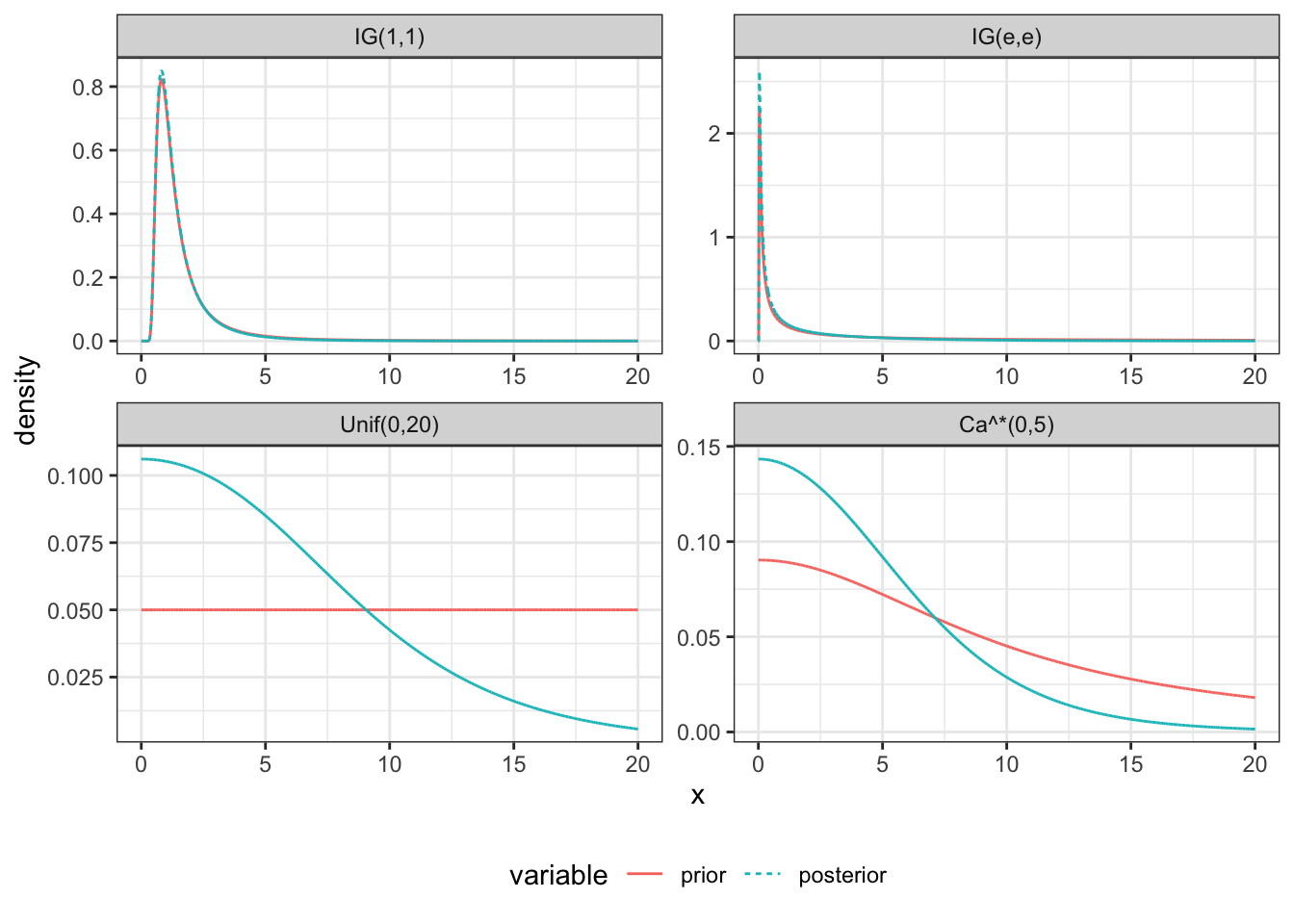

Posterior Predictive Checks

Let $y^{rep}$ be a replication of $y$, then $$p(y^{rep}|y) = \int p(y^{rep}|\theta,y) p(\theta|y) d\theta = \int p(y^{rep}|\theta) p(\theta|y) d\theta.$$ where $y$ is the observed data and $\theta$ are the model parameters.

To simulate a full replication:

1. Simulate $\theta^{(j)} \sim p(\theta\mid y)$ and
2. Simulate $y^{rep,j} \sim p(y\mid \theta^{(j)})$

To assess model adequacy:

• Compare plots of replicated data to the observed data.
• Calculate posterior predictive p-values.
  • Define a test statistic $T(y, \theta)$
  • Define the posterior predictive p-value: $p_B = P(T(y^{rep}, \theta)) \geq T(y, \theta) \mid y)$
  • Small or large p-values are (possible) cause for concern