5.4 Convex Optimisation

Definition 5.1 (convex optimization problem) According to (Boyd, Boyd, and Vandenberghe 2004), the general form is: \[ \begin{array}{ll} \operatorname{minimize} & f_{0}(x) \\ \text { subject to } & f_{i}(x) \leq b_{i}, \quad i=1, \ldots, m \end{array} \] where the functions \(f_{0}, \ldots, f_{m}: \mathbf{R}^{n} \rightarrow \mathbf{R}\) are convex.

Recognizing convex optimization problems, or those that can be transformed to convex optimization problems, can therefore be challenging. (Boyd, Boyd, and Vandenberghe 2004)

5.4.1 Convex or Concave Functions

Definition 5.2 \(f\left(x_{1}, x_{2}, \ldots, x_{n}\right)\) is a convex function if, for each pair of points on the graph of \(f\left(x_{1},\right.\) \(\left.x_{2}, \ldots, x_{n}\right),\) the line segment joining these two points lies entirely above or on the graph of \(f\left(x_{1},\right.\) \(\left.x_{2}, \ldots, x_{n}\right) .\) It is a strictly convex function if this line segment actually lies entirely above this graph except at the endpoints of the line segment. Concave functions and strictly concave functions are defined in exactly the same way, except that above is replaced by below. (Hillier 2012)

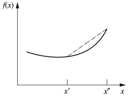
Figure 5.1: A strictly convex function.

The sum of convex functions is a convex function, and the sum of concave functions is a concave function. (Hillier 2012)

Definition 5.3 (Hessian Matrix) (Morgan 2015) The Hessian matrix of a twice-differentiable function is a matrix array of all of the function’s second-order derivatives. Specifically, if \(f\left(x_{1}, \ldots, x_{n}\right)\) is a function that is differentiable to order 2, then the function’s Hessian matrix is the array of functions: \[ H_{f}(x)=\left(\begin{array}{cccc} \frac{\partial^{2} f}{\partial x_{1}^{2}} & \frac{\partial^{2} f}{\partial x_{1} \partial x_{2}} & \cdots & \frac{\partial^{2} f}{\partial x_{1} \partial x_{n}} \\ \frac{\partial^{2} f}{\partial x_{2} \partial x_{1}} & \frac{\partial^{2} f}{\partial x_{2}^{2}} & \cdots & \frac{\partial^{2} f}{\partial x_{2} \partial x_{n}} \\ \vdots & \vdots & \ddots & \vdots \\ \frac{\partial^{2} f}{\partial x_{n} \partial x_{1}} & \frac{\partial^{2} f}{\partial x_{n} \partial x_{2}} & \cdots & \frac{\partial^{2} f}{\partial x_{n}^{2}} \end{array}\right) \]

Convexity Test for Multi-Variate Function

In mathematical terminology, \(f\left(x_{1}, x_{2}, \ldots, x_{n}\right)\) is convex if and only if its \(n \times n\) Hessian matrix is positive semidefinite for all possible values of \(\left(x_{1}, x_{2}, \ldots, x_{n}\right)\). (Hillier 2012)

\[ \begin{array}{ccccc} \hline & \text { Strictly } & & \text { Strictly } \\ \text { Quantity } & \text { Convex } & \text { Convex } & \text { Concave } & \text { Concave } \\ \hline \frac{\partial^{2} f\left(x_{1}, x_{2}\right)}{\partial x_{1}^{2}} \frac{\partial^{2} f\left(x_{1}, x_{2}\right)}{\partial x_{2}^{2}}-\left[\frac{\partial^{2} f\left(x_{1}, x_{2}\right)}{\partial x_{1} \partial x_{2}}\right]^{2} & \geq 0 & >0 & \geq 0 & >0 \\ \frac{\partial^{2} f\left(x_{1}, x_{2}\right)}{\partial x_{1}^{2}} & \geq 0 & >0 & \leq 0 & <0 \\ \frac{\partial^{2} f\left(x_{1}, x_{2}\right)}{\partial x_{2}^{2}} & \geq 0 & >0 & \leq 0 & <0 \\ \hline \end{array} \]

5.4.2 Convex Set

Definition 5.4 A convex set is a collection of points such that, for each pair of points in the collection, the entire line segment joining these two points is also in the collection. (Hillier 2012)

5.4.3 Regularity Conditions (Constraint Qualifications)

There are many results that establish conditions on the problem, beyond convexity, under which strong duality holds. These conditions are called constraint qualifications. (Boyd, Boyd, and Vandenberghe 2004)

In mathematics, Slater’s condition (or Slater condition) is a sufficient condition for strong duality to hold for a convex optimisation problem.

If a convex optimization problem with differentiable objective and constraint functions satisfies Slater’s condition, then the KKT conditions provide necessary and sufficient conditions for optimality. (Boyd, Boyd, and Vandenberghe 2004)

5.4.4 Lagrangian Duality

There also are many valuable indirect applications of the KKT conditions. One of these applications arises in the duality theory that has been developed for nonlinear programming to parallel the duality theory for linear programming. (Hillier 2012)

The basic idea in Lagrangian duality is to take the constraints in (5.1) into account by augmenting the objective function with a weighted sum of the constraint functions.

For example: \[ \begin{align} \max_{\mathbf{x}} \quad & f(\mathbf{x})\\ \text{s.t.} \quad & \boldsymbol{g}(\boldsymbol{x}) \leq \mathbf{0} \\ & \boldsymbol{h}(\boldsymbol{x}) = \mathbf{0} \end{align} \]

The dual problem is \[ \begin{align} \min_{\boldsymbol{u}, \boldsymbol{v}} \quad & \theta(\boldsymbol{u}, \boldsymbol{v}) \\ \text{s.t.} \quad & \boldsymbol{u} \geq 0 \end{align} \] where \[ \theta(\boldsymbol{u}, \boldsymbol{v}) = \max _{\boldsymbol{x}} \{f(\boldsymbol{x}) + \boldsymbol{u} \boldsymbol{g}(\boldsymbol{x}) + \boldsymbol{v} \boldsymbol{h}(\boldsymbol{x}) \} \]

References

Boyd, Stephen, Stephen P Boyd, and Lieven Vandenberghe. 2004. Convex Optimization. Cambridge university press.

Hillier, Frederick S. 2012. Introduction to Operations Research. Tata McGraw-Hill Education.

Morgan, Peter B. 2015. An Explanation of Constrained Optimization for Economists. University of Toronto Press.