14.3 Optimal Power Flow (OPF)

Different levels are needed.

Congestion in the transmission network can therefore transform a reasonably competitive global market into a collection of smaller local energy markets. (Kirschen and Strbac 2018)

At the heart of most power system optimizations are the equations of the steady-state, single-phase approximation to alternating current power flow in a network. Well-known problems like optimal power flow, reconfiguration, and transmission planning all consist of details layered on top of power flow. Nodal prices, a core component of electricity markets, are obtained from the dual of optimal power flow. It is therefore most unfortunate that the power flow equations are nonconvex, making all of these optimizations extremely difficult. We are thus faced with a tradeoff between realistic models that are too hard to solve at practical scales and tractable approximations. (Taylor 2015)

14.3.1 Models and Algorithms

This book only contains models and, with the exception of Chapters 2 and 7 , rarely mentions algorithms. This is not because the algorithms are not worth knowing or decoupled from modeling; one can always do better by formulating optimization models and algorithms jointly. Rather, here this wisdom is applied by formulating models so that they can be solved by certain algorithms. This approach is a luxury we can afford because optimization is a relatively mature field: for a desired level of scalability, it identifies the corresponding tradeoff between efficiency and descriptiveness. (Taylor 2015)

In words, optimal power flow is the problem of minimizing some function of voltage, current, and power, subject to the resulting flow being able to feasibly traverse a transmission or distribution system. System operators solve optimal power flow routines to do long-term planning, days- to hour-ahead scheduling, real-time dispatch, and pricing (to name a few), making it one of the most frequently employed optimization routines in power systems. (Taylor 2015)

Definition 14.1 (nonconvex quadratically constrained power flow problem) The problem can be written as: \[ \begin{align} \min_{v, p, q} \quad & f(v, p, q) \\ \text{s.t.} \quad & p_{i j}+i q_{i j}=v_{i}\left(v_{i}^{*}-v_{j}^{*}\right) y_{i j}^{*} \tag{14.1} \\ & \sum_{j} p_{i j}=p_{i} \\ & \sum_{j} q_{i j}=q_{i} \\ & \underline{p}_{i} \leq p_{i} \leq \bar{p}_{i} \\ & q_{i} \leq q_{i} \leq \bar{q}_{i} \\ & p_{i j}^{2}+q_{i j}^{2} \leq \bar{s}_{i j}^{2} \\ & \underline{v}_{i} \leq\left|v_{i}\right| \leq \bar{v}_{i} \end{align}\]

Note that optimal power flow is a steady-state formulation. From a simulation perspective, this description of power system physics is therefore rather minimal in that it omits dynamics, harmonics, and load models, to name a few; moreover, the above is relatively simple even among optimal power flow formulations in that it also omits transformer tap positions and other fine-grained control variables. On the other hand, it is already hovering around the upper tractable limit of optimization, and this is entirely due to (14.1) a (nonconvex) quadratic equality constraint.

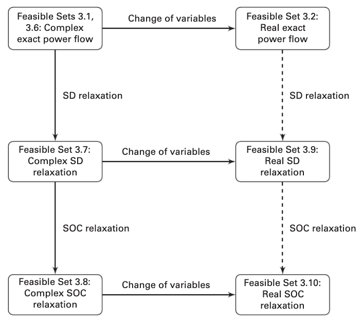
Figure 14.1: Relationships among power flow relaxations.

14.3.2 Centralized Trading

The nodal marginal price is equal to the cost of supplying an additional megawatt of load at the node under consideration by the cheapest possible means while respecting the constraints imposed by the network capacity limits. (Kirschen and Strbac 2018)

14.3.3 Security-Constrained Unit Commitment (SCUC)

14.3.4 Steady-State Power Network Optimization

14.3.5 Load Flow

Chapter 11 Load Flow in (???)

References

Kirschen, Daniel S, and Goran Strbac. 2018. Fundamentals of Power System Economics. John Wiley & Sons.

Taylor, Joshua Adam. 2015. Convex Optimization of Power Systems. Cambridge University Press.