5 Finding Meaningful Clusters of Matches
Next, we might be interested in finding meaningful “archetypes” of games, based on variables in the gamelog dataset. We omit the games for which only one innings data is available to reduce the likelihood of bias.
innings_check <- gamelog %>% dplyr::group_by(MatchNo) %>%
                 dplyr::summarise(innings=sum(length(unique(Inning))==2) + 1)

match_data = ddply(subset(gamelog,MatchNo %in% innings_check$MatchNo[innings_check$innings==2]),
                   "MatchNo",summarize,
                   home_runs= sum(NumOutcome[NumOutcome > 0 & Inning==1]),
                   away_runs= sum(NumOutcome[NumOutcome > 0 & Inning==2]),
                   home_wickets= 0-sum(NumOutcome[NumOutcome < 0 & Inning==1]),
                   away_wickets= 0-sum(NumOutcome[NumOutcome < 0 & Inning==2]),
                   total_wickets = 0 -sum(NumOutcome[NumOutcome < 0]),
                   home_overs = max(Over[Inning==1]),
                   away_overs = max(Over[Inning==2]),
                   home_balls = length(Ball[Inning==1]),
                   away_balls = length(Ball[Inning==2]),
                   home_balls_till_1st_wicket = length(which(Wickets==0 & Inning==1)),
                   away_balls_till_1st_wicket = length(which(Wickets==0 & Inning==2)),
                   home_sixes = sum(NumOutcome[NumOutcome==6 & Inning==1])/6,
                   away_sixes = sum(NumOutcome[NumOutcome==6 & Inning==2])/6,
                   total_sixes = sum(NumOutcome[NumOutcome==6])/6,
                   excitement = mean(Sentiment))
We first look at clusters based on runs scored by the team batting in the first innings (“home” side) and the number of balls faced by the away side. We proceed to plot an elbow plot:
wssd <- rep(0,9)
for (k in 2:10) {
  set.seed(123)
  clust <- kmeans(subset(match_data,away_balls > 50,c(home_runs,away_balls)),centers=k)
  wssd[k-1] <- clust$tot.withinss
}
centers <- 2:10
dat <- data.frame(centers,wssd)

ggplot(dat,aes(centers,wssd)) + geom_line() + geom_point()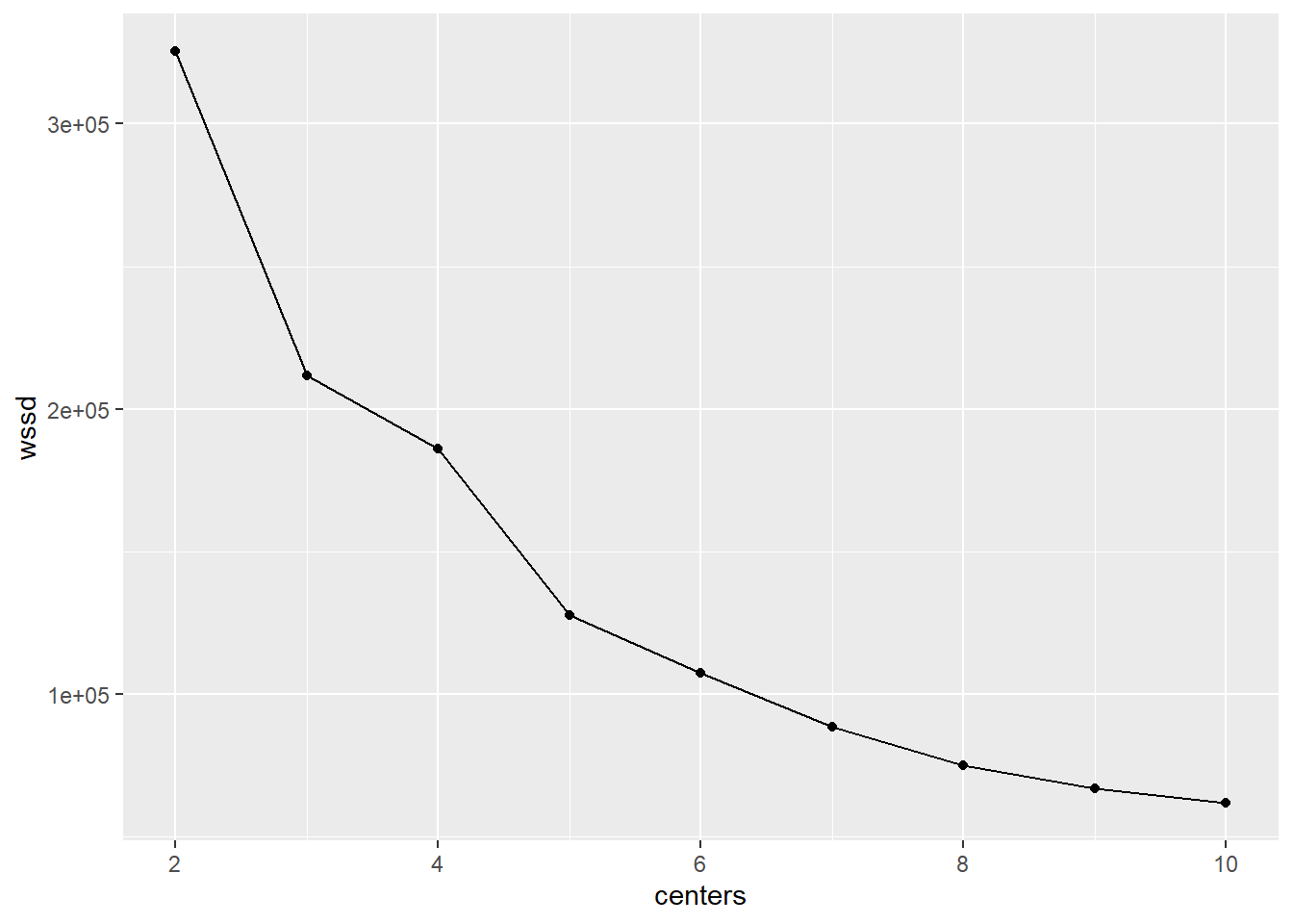
There are two candidates for an appropriate number of clusters here - 3 and 5, since these are the points at which the slopes of lines change most dramatically. We opt for 5 since this is a better fit and will be more informative while still being parsimonious.
set.seed(123)
ggplot(subset(match_data,away_balls > 50),aes(home_runs,away_balls)) + geom_density_2d_filled()+
  geom_point(colour='white',alpha=0.2) + geom_point(data=as.data.frame(kmeans(subset(match_data,away_balls > 50,c(home_runs,away_balls)),centers=5)$centers),col='red',size=5,pch=as.character(1:5)) +
  geom_abline(slope=0,intercept = 120,colour='white',linetype='dashed')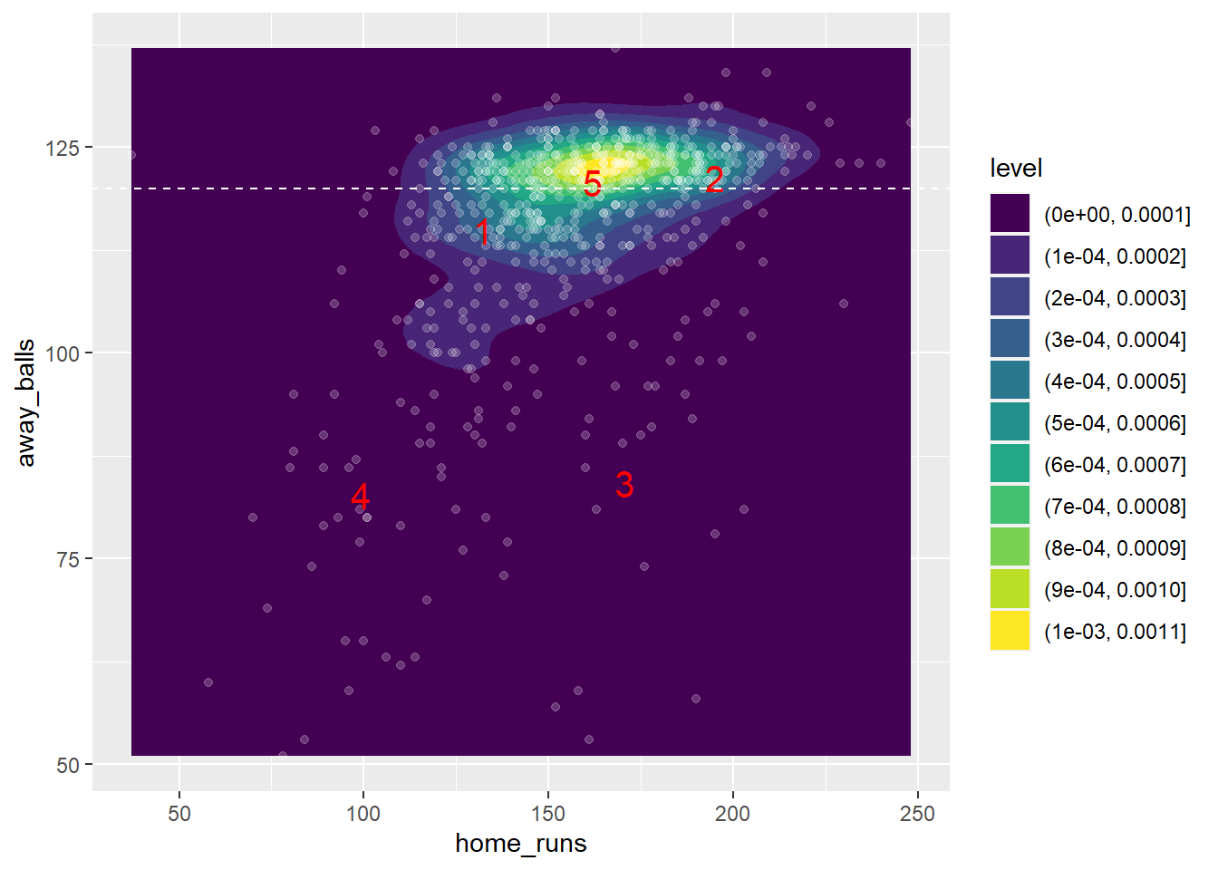
We find five main kinds of games here, with their centres identifiable on the above plot as large red points. Note the dashed white horizontal line is at 120 balls played in the second innings, i.e. a full 20 overs (less a few replayed balls):
Cluster 1 is characterized by a less-than-average to average number of runs scored by the home team (125-150) and slightly less than 120 balls played in the second innings - this represents a low-scoring match edged by the away team (most of the time, or there is a possibility that they lost by losing all their wickets, but this is rarer, occurring in only 10% of the second innings in our data)
Cluster 2 corresponds to a type of match in which the home team scores a high number of runs (at least 175, on average 190) and all 20 overs are played. This can be a high-scoring victory for the home team or a narrow high-scoring victory for the away team.
Cluster 3 corresponds to a match in which the home team scores slightly more than average runs (~ 170) and the away team faced well below 120 balls (around 80). This kind of game can be one in which the away team lost all 10 wickets and were comfortably beaten by the home team, or a game that was interrupted or for which there is incomplete data, or even a high-scoring game in which the away team raced to a high number of runs in under 17 overs.
Cluster 4 is characterized by a low number of runs scored by the home team (less than 125, 100 on average) and less than 20 overs played by the away team (80 balls on average). This is a cluster consisting of mostly comfortable, low-scoring victories for the away side.
Cluster 5 is the most typical kind of game, i.e. one in which the team batting first scores an average number of runs (140-170, 155 on average) and the full 20 overs (or close to that) are played. This can be a narrow victory for either side with a typical number of runs scored, or even a blowout victory for the home side in which the away side scores very few runs.
Next, we look for clusters based on sixes scored, wickets,and excitement.
wssd <- rep(0,9)
for (k in 2:10) {
set.seed(123)
clust <- kmeans(subset(match_data,select=c(total_sixes,total_wickets,excitement)),centers=k)
wssd[k-1] <- clust$tot.withinss
}
centers <- 2:10
dat <- data.frame(centers,wssd)
ggplot(dat,aes(centers,wssd)) + geom_line() + geom_point()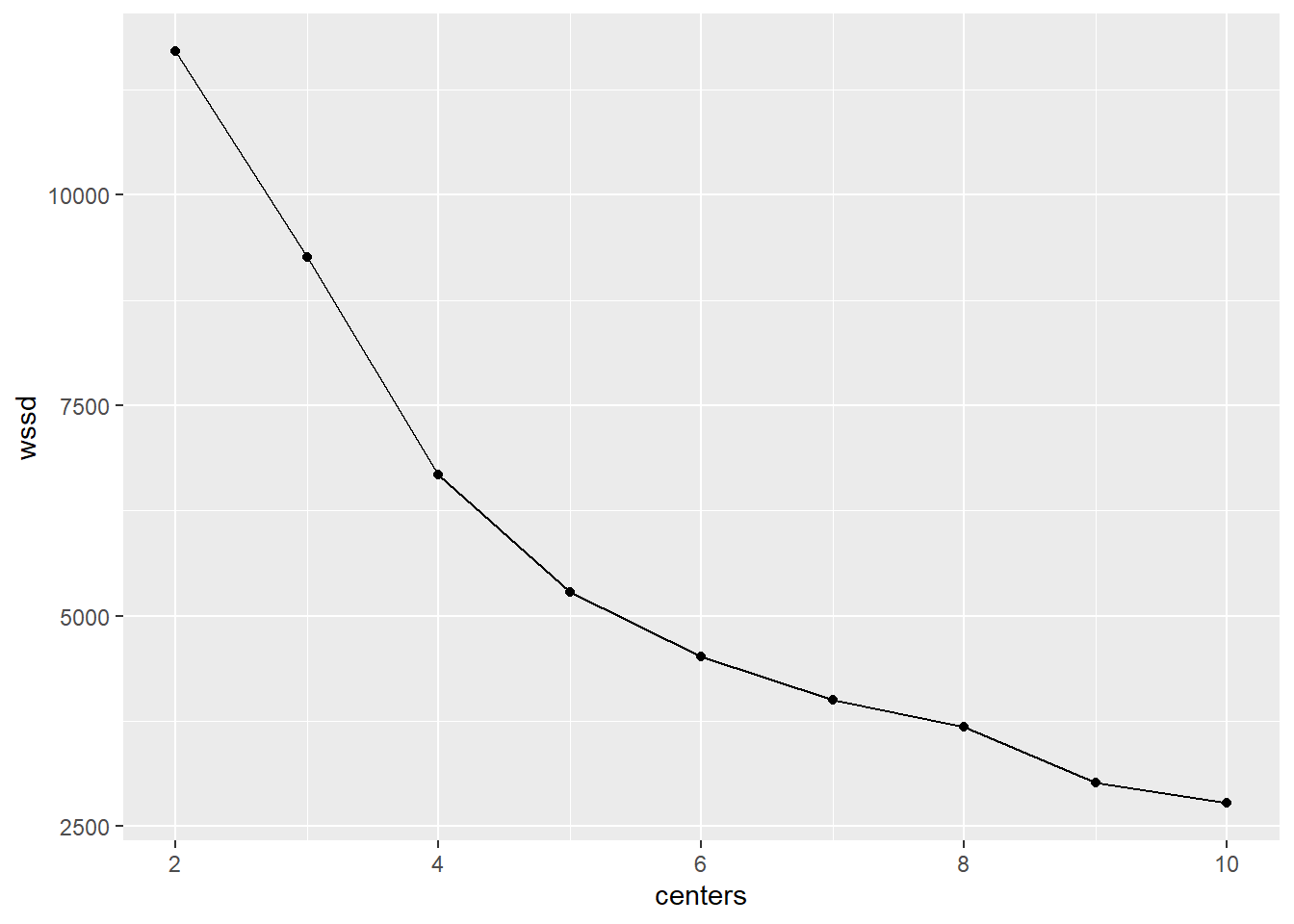 Althought there is no clear elbow, 5 looks to be the best choice here as it has the best balance of parsimony and goodness-of-fit.
set.seed(123)
ggplot(match_data,aes(total_sixes,total_wickets,fill=excitement)) +
geom_tile() + geom_point(data=as.data.frame(kmeans(subset(match_data,
select=c(total_sixes,total_wickets,excitement)),centers=5)$centers),col='red',size=5,pch=as.character(1:5)) +
scale_fill_viridis_b()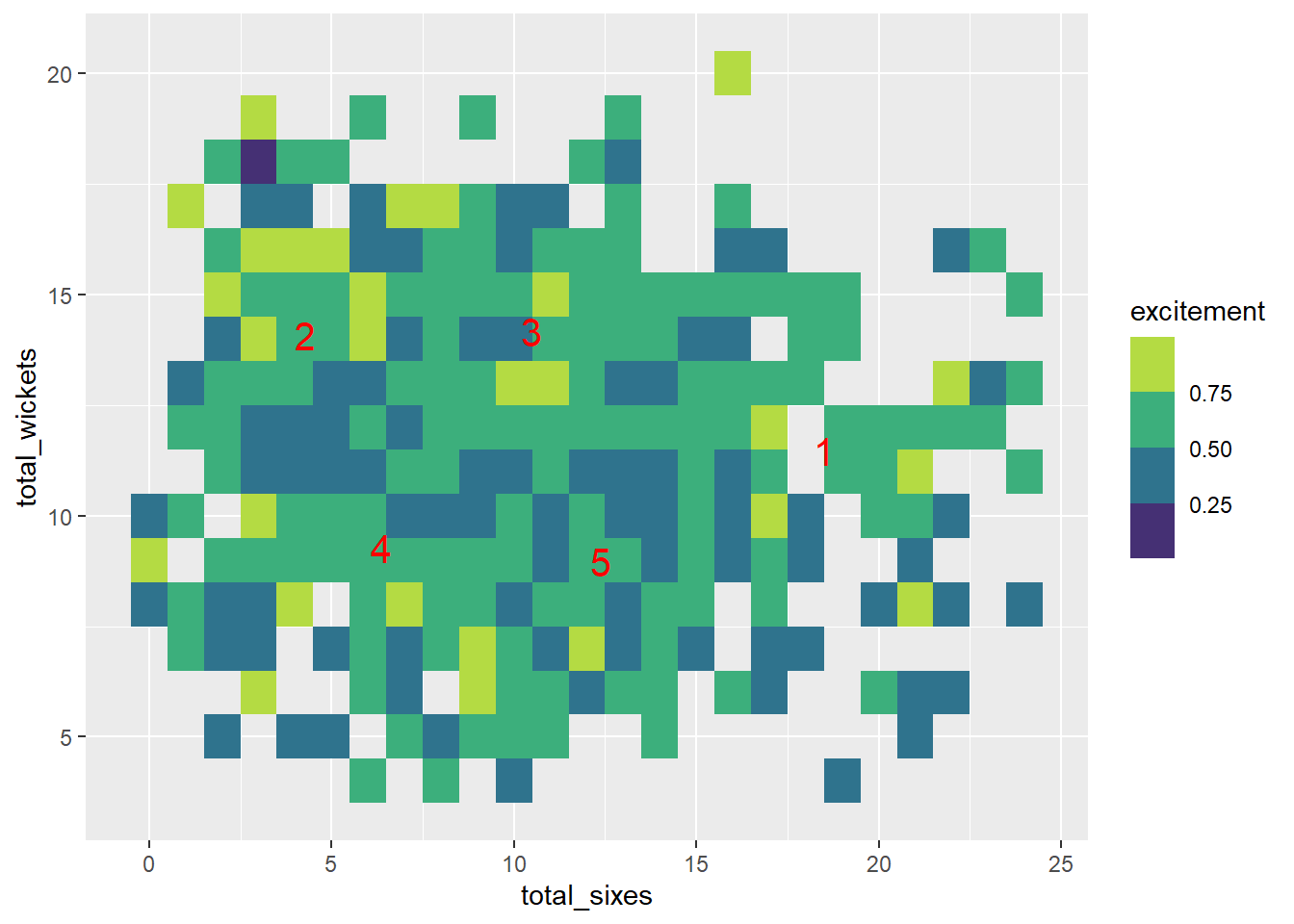 The 5 clusters are characterized as follows
- Cluster 1 has a high number of sixes and an average number of wickets. The excitement level is in the second highest quartile on average.
- Cluster 2 has a low number of sixes and slightly higher than average number of wickets. It has the most number of entertaining matches (i.e. top-quartile excitement) out of all the clusters as well as the most number of dull matches (2nd-lowest quantile)
- Cluster 3 has an average number of sixes and slightly higher than average number of wickets, and its excitement level is mostly in the second highest quartile.
- Cluster 4 has low wickets, low sixes, and average excitement.
- Cluster 5 has an average number of sixes and wickets, and a low-to-average excitement.