Chapter 2 Exercicio
- Considere os conjuntos de dados house price cenário 1 e cenário 2.
- Faça uma análise descritiva para ambos os conjuntos. O que se pode notar de diferente?
- Ajuste um modelo de regressão linear simples para ambos conjuntos no qual o valor seja explicado pela a área. Discuta.
- Se uma casa possuir 1300 ft², qual seria o preço esperado de acordo com o modelo do cenário 1? E de acordo com o modelo do cenário 2?
2.1 Análise descritiva - Cenário 1
Coletando os dados
library(readxl)
cenario1 = read_excel("Dados/Data_HousePrice_Area.xlsx", sheet = "Cenario 1")
print(cenario1)
## # A tibble: 10 × 2
## `Square Feet` `House Price`
## <dbl> <dbl>
## 1 1400 245
## 2 1600 312
## 3 1700 279
## 4 1875 308
## 5 1100 199
## 6 1550 219
## 7 2350 405
## 8 2450 324
## 9 1425 319
## 10 1700 255price=cenario1$`House Price`
square=cenario1$`Square Feet`
print(price)## [1] 245 312 279 308 199 219 405 324 319 255print(square)## [1] 1400 1600 1700 1875 1100 1550 2350 2450 1425 1700plot(price,square,main="Dispersão do Preço de Casa por Área")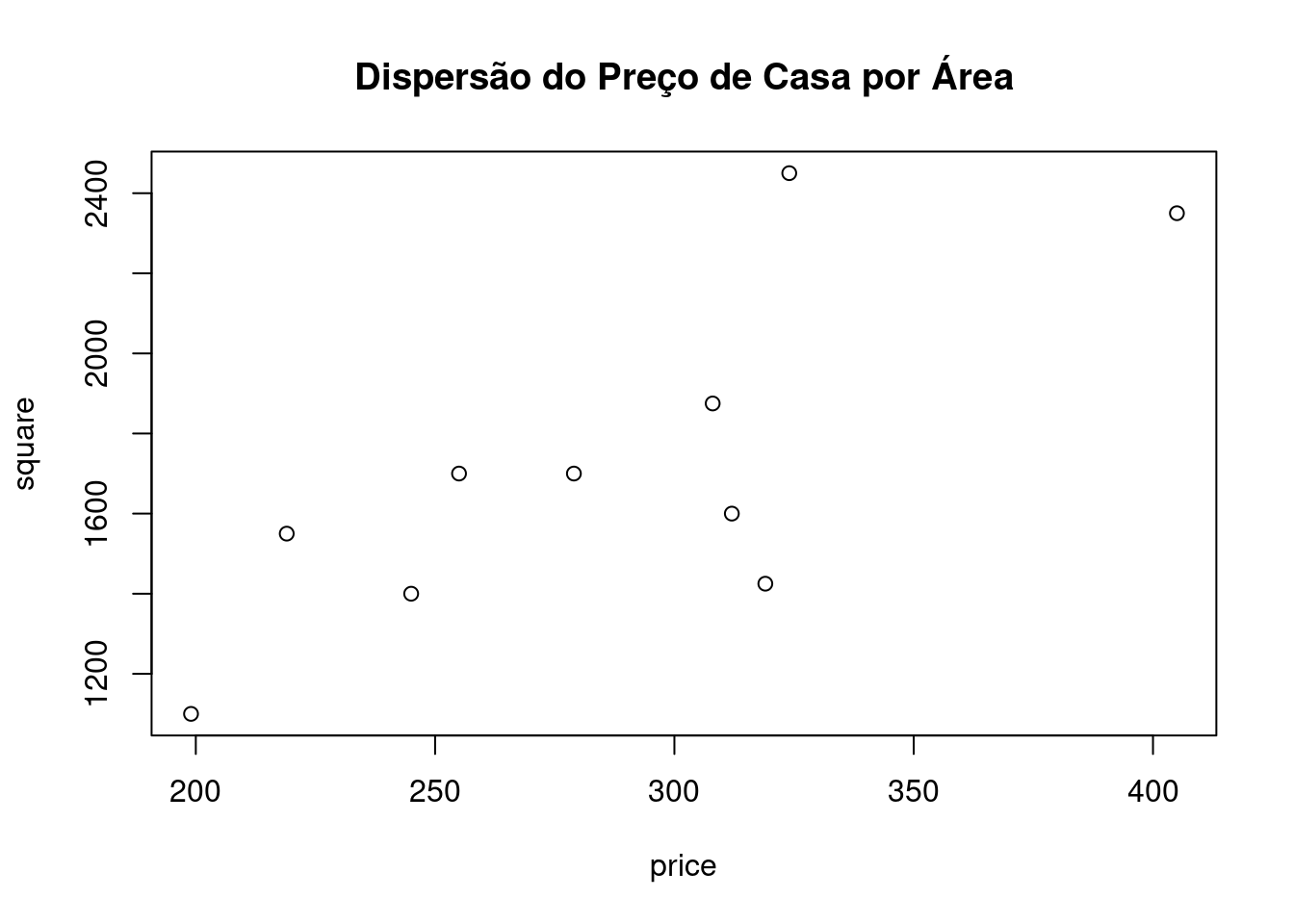
2.2 Análise descritiva - Cenario 2
Leitura da base de Dados
cenario2 = read_excel("Dados/Data_HousePrice_Area.xlsx", sheet = "Cenario 2")
print(cenario2)
## # A tibble: 10 × 2
## `Square Feet` `House Price`
## <dbl> <dbl>
## 1 1400 245
## 2 1800 312
## 3 1700 279
## 4 1875 308
## 5 1200 199
## 6 1480 219
## 7 2350 405
## 8 2100 324
## 9 2000 319
## 10 1700 255plot(cenario2,main="Dispersão do Preço de Casas por Area - Cenario 2")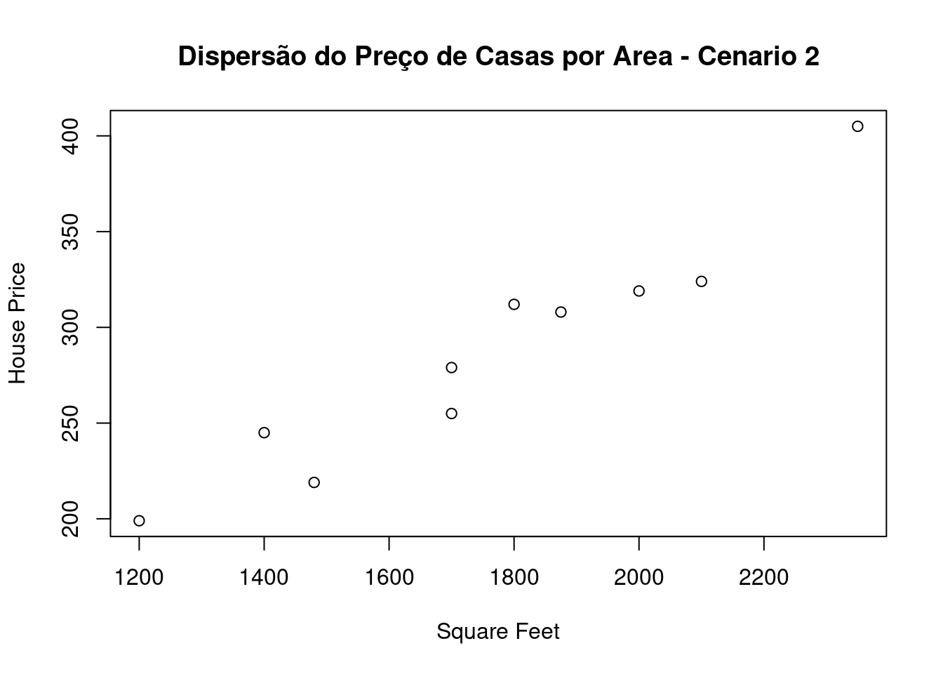
2.3 Gráfico de dispersão
Montagem do gráfico de dispersão para os dois cenários, comparando o preço da casa e sua área
par(mfrow = c(1,2))
plot(cenario1, col = 2, pch = 16, xlab = "Area", ylab = "Preco", main = "Cenário 1")
plot(cenario2, col = 3, pch = 17, xlab = "Area", ylab = "Preco", main = "Cenário 2")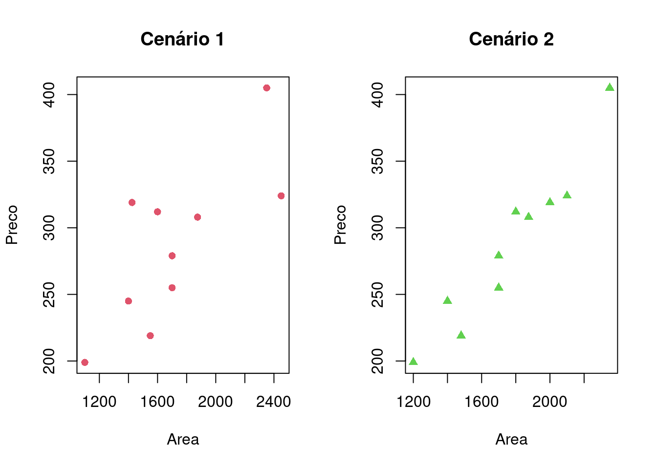
Nao e possivel identificar um padrao em funcao dos valores apresentados.
O Cenario 2 demonstra os valores proximos a uma reta e nao demonstra valores de formaexpalhados como ocorre no Cenario 1
2.4 Modelo de Regresão Linear
A regressão tem como objetivo Medir a influência de uma ou mais variáveis X sobre a Variavel Y., Nesse caso X e explicativa e Y e quem responde tal influencia.
modelo_Cenario1 = lm(`House Price` ~ `Square Feet`, data = cenario1)
summary(modelo_Cenario1)
##
## Call:
## lm(formula = `House Price` ~ `Square Feet`, data = cenario1)
##
## Residuals:
## Min 1Q Median 3Q Max
## -49.388 -27.388 -6.388 29.577 64.333
##
## Coefficients:
## Estimate Std. Error t value Pr(>|t|)
## (Intercept) 98.24833 58.03348 1.693 0.1289
## `Square Feet` 0.10977 0.03297 3.329 0.0104 *
## ---
## Signif. codes: 0 '***' 0.001 '**' 0.01 '*' 0.05 '.' 0.1 ' ' 1
##
## Residual standard error: 41.33 on 8 degrees of freedom
## Multiple R-squared: 0.5808, Adjusted R-squared: 0.5284
## F-statistic: 11.08 on 1 and 8 DF, p-value: 0.01039modelo_Cenario2 = lm(`House Price` ~ `Square Feet`, data = cenario2)
summary(modelo_Cenario2)##
## Call:
## lm(formula = `House Price` ~ `Square Feet`, data = cenario2)
##
## Residuals:
## Min 1Q Median 3Q Max
## -21.323 -16.654 2.458 15.838 19.336
##
## Coefficients:
## Estimate Std. Error t value Pr(>|t|)
## (Intercept) -9.64509 30.46626 -0.317 0.76
## `Square Feet` 0.16822 0.01702 9.886 9.25e-06 ***
## ---
## Signif. codes: 0 '***' 0.001 '**' 0.01 '*' 0.05 '.' 0.1 ' ' 1
##
## Residual standard error: 17.56 on 8 degrees of freedom
## Multiple R-squared: 0.9243, Adjusted R-squared: 0.9149
## F-statistic: 97.73 on 1 and 8 DF, p-value: 9.246e-062.4.1 Aplicando a reta de regresão no Grafico
par(mfrow = c(1,2))

plot(cenario1$`House Price` ~ cenario1$`Square Feet`, col = 2, pch = 16, xlab = "Area", ylab = "Preço", main = "Cenário 1")
abline(modelo_Cenario1, col = 1, lwd = 2)
plot(cenario2$`House Price` ~ cenario2$`Square Feet`, col = 3, pch = 17, xlab = "Area", ylab = "Preço", main = "Cenário 2")
abline(modelo_Cenario2, col = 1, lwd = 2)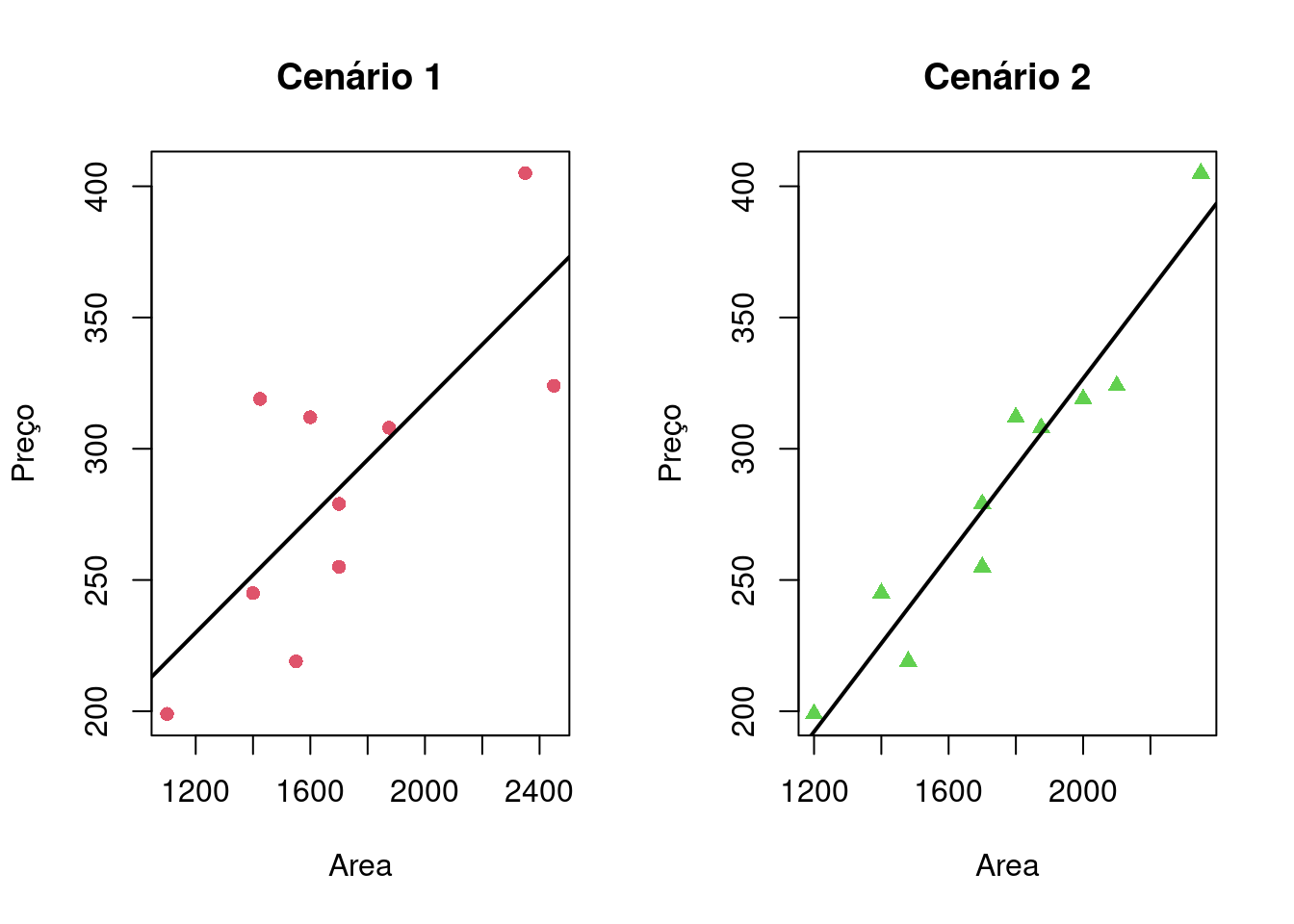
Comparando ambos os gráfico pode-se notar que o primeiro conjunto é mais espacado e o segundo possui o cenário de dados agrupados de forma linear.
Se uma casa possuir 1300 ft², qual seria o preço esperado de acordo com o modelo do cenário 1?
Area = 1300
Modelo = round(modelo_Cenario1$coefficients[1] + Area * modelo_Cenario1$coefficients[2])
print( Modelo )
## (Intercept)
## 2412.5 Predição, Regressao e Classificacao
modelo_Cen02 <- lm(cenario2$`Square Feet` ~ cenario2$`House Price`)
modelo_Cen02
##
## Call:
## lm(formula = cenario2$`Square Feet` ~ cenario2$`House Price`)
##
## Coefficients:
## (Intercept) cenario2$`House Price`
## 186.202 5.495Cálculo do resíduo:
\(y = 186.202 + 5.495 x\) para \(x = 1400\), \(y = valor\). Considerando que a diferença entre o y dado e o calculado sera o resíduo apresentado.
resumocenario02 = summary(cenario2)
resumocenario02
## Square Feet House Price
## Min. :1200 Min. :199.0
## 1st Qu.:1535 1st Qu.:247.5
## Median :1750 Median :293.5
## Mean :1760 Mean :286.5
## 3rd Qu.:1969 3rd Qu.:317.2
## Max. :2350 Max. :405.0Neste cenário as observações estão mais agrupadas próximas a uma reta, o modelo linear simples descreveu melhor as observações.
p = predict(modelo_Cen02, novoresulado = data.frame(x = 1300))2.5.2 Pacotes
Pacotes necessários para estes exercícios:
library(readxl)
library(tidyverse)
library(readxl)
library(ggthemes)
library(plotly)
library(knitr)
library(kableExtra)
library(factoextra)
2.5.3 Conjunto de dados
Considere os dados a seguir do consumo alimentar médio de diferentes tipos de alimentos para famílias classificadas de acordo com o número de filhos (2, 3, 4 ou 5) e principal área de trabalho (MA: Setor de Trabalho Manual, EM: Empregados do Setor Público ou CA: Cargos Administrativos).
Fonte: LABORATORIO-R.pdf
dados = tibble(AreaTrabalho = as.factor(rep(c("MA", "EM", "CA"), 4)),
               Filhos = as.factor(rep(2:5, each = 3)),
               Paes = c(332, 293, 372, 406, 386, 438, 534, 460, 385, 655, 584, 515),
               Vegetais = c(428, 559, 767, 563, 608, 843, 660, 699, 789, 776, 995, 1097),
               Frutas = c(354, 388, 562, 341, 396, 689, 367, 484, 621, 423, 548, 887),
               Carnes = c(1437,1527,1948,1507,1501,2345,1620,1856,2366,1848,2056,2630),
               Aves = c(526, 567, 927, 544, NA, 1148,638, 762, 1149,759, 893, 1167),
               Leite = c(247, 239, 235, 324, 319, 243, 414, 400, 304, 495, 518, 561),
               Alcoolicos = c(427, 258, 433, 407, 363, 341, 407, 416, 282, 486, 319, 284))

kable(dados) %>%
  kable_styling(latex_options = "striped")
2.5.4 Regressão
#dummy <- dummyVars(" ~ .", data=dados)
#dadosS <- data.frame(predict(dummy, newdata = dados))
dadosS = subset(dados, select=c("Aves", "Filhos", "Paes", "Vegetais", "Frutas", "Carnes", "Leite", "Alcoolicos"))

#modelo  = lm(dadosS$Aves ~ dadosS$AreaTrabalho.CA + dadosS$AreaTrabalho.EM + dadosS$AreaTrabalho.MA + dadosS$Filhos.2 + dadosS$Filhos.3 + dadosS$Filhos.4 + dadosS$Filhos.5 + dadosS$Paes + dadosS$Vegetais + dadosS$Frutas + dadosS$Carnes + dadosS$Leite + dadosS$Alcoolicos)

modelo  = lm(Aves ~ Filhos + Paes + Vegetais + Frutas + Carnes + Leite + Alcoolicos, data = dadosS)

valoresPredito = predict.lm(modelo, type = "response")
summary(modelo)
##
## Call:
## lm(formula = Aves ~ Filhos + Paes + Vegetais + Frutas + Carnes +
## Leite + Alcoolicos, data = dadosS)
##
## Residuals:
## 1 2 3 4 6 7 8 9 10 11 12
## 11.874 -9.816 -2.058 -1.250 1.250 3.533 -5.322 1.789 -8.056 9.567 -1.510
##
## Coefficients:
## Estimate Std. Error t value Pr(>|t|)
## (Intercept) -746.3706 632.2722 -1.180 0.447
## Filhos3 -75.6290 123.1415 -0.614 0.649
## Filhos4 -105.4167 262.6281 -0.401 0.757
## Filhos5 -192.0193 421.1901 -0.456 0.728
## Paes 0.1803 0.3299 0.547 0.681
## Vegetais 0.2438 0.2282 1.068 0.479
## Frutas -0.7431 0.9391 -0.791 0.574
## Carnes 0.9335 0.5221 1.788 0.325
## Leite -0.1543 1.1509 -0.134 0.915
## Alcoolicos 0.1313 0.2243 0.586 0.663
##
## Residual standard error: 21.15 on 1 degrees of freedom
## (1 observation deleted due to missingness)
## Multiple R-squared: 0.9993, Adjusted R-squared: 0.9928
## F-statistic: 153.7 on 9 and 1 DF, p-value: 0.06252confint(modelo)## 2.5 % 97.5 %
## (Intercept) -8780.151071 7287.409914
## Filhos3 -1640.289906 1489.031864
## Filhos4 -3442.422544 3231.589190
## Filhos5 -5543.747107 5159.708466
## Paes -4.010944 4.371643
## Vegetais -2.655840 3.143461
## Frutas -12.674990 11.188748
## Carnes -5.701068 7.567978
## Leite -14.778470 14.469823
## Alcoolicos -2.718471 2.981129rse = sigma(modelo)/mean(dadosS$Aves, na.rm = TRUE)
rse## [1] 0.02562551plot(dadosS, pch = 16, col = "blue") #Plot the results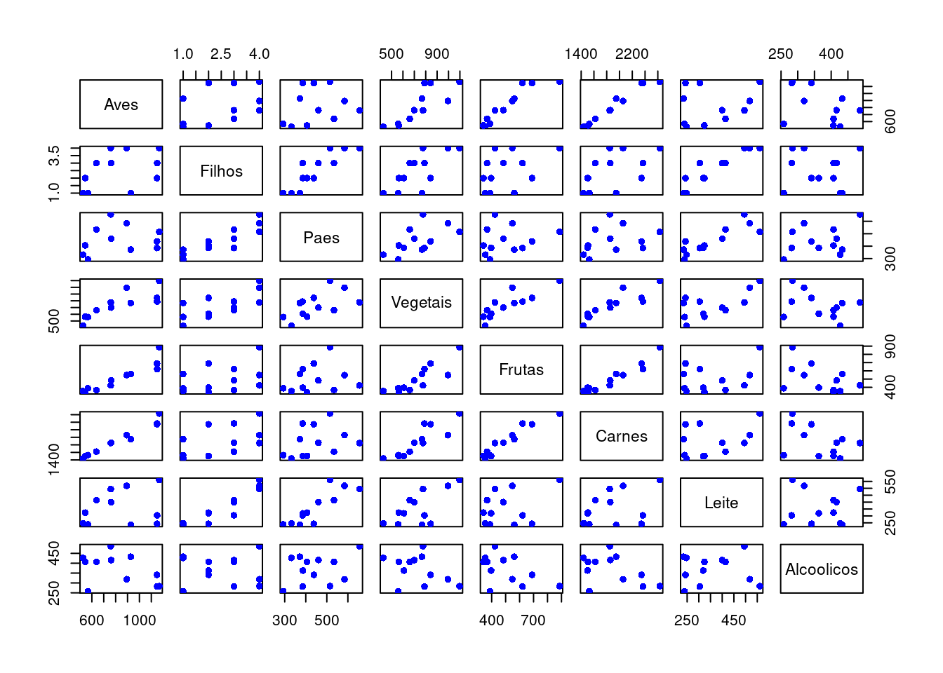
plot(modelo$residuals, pch = 16, col = "red")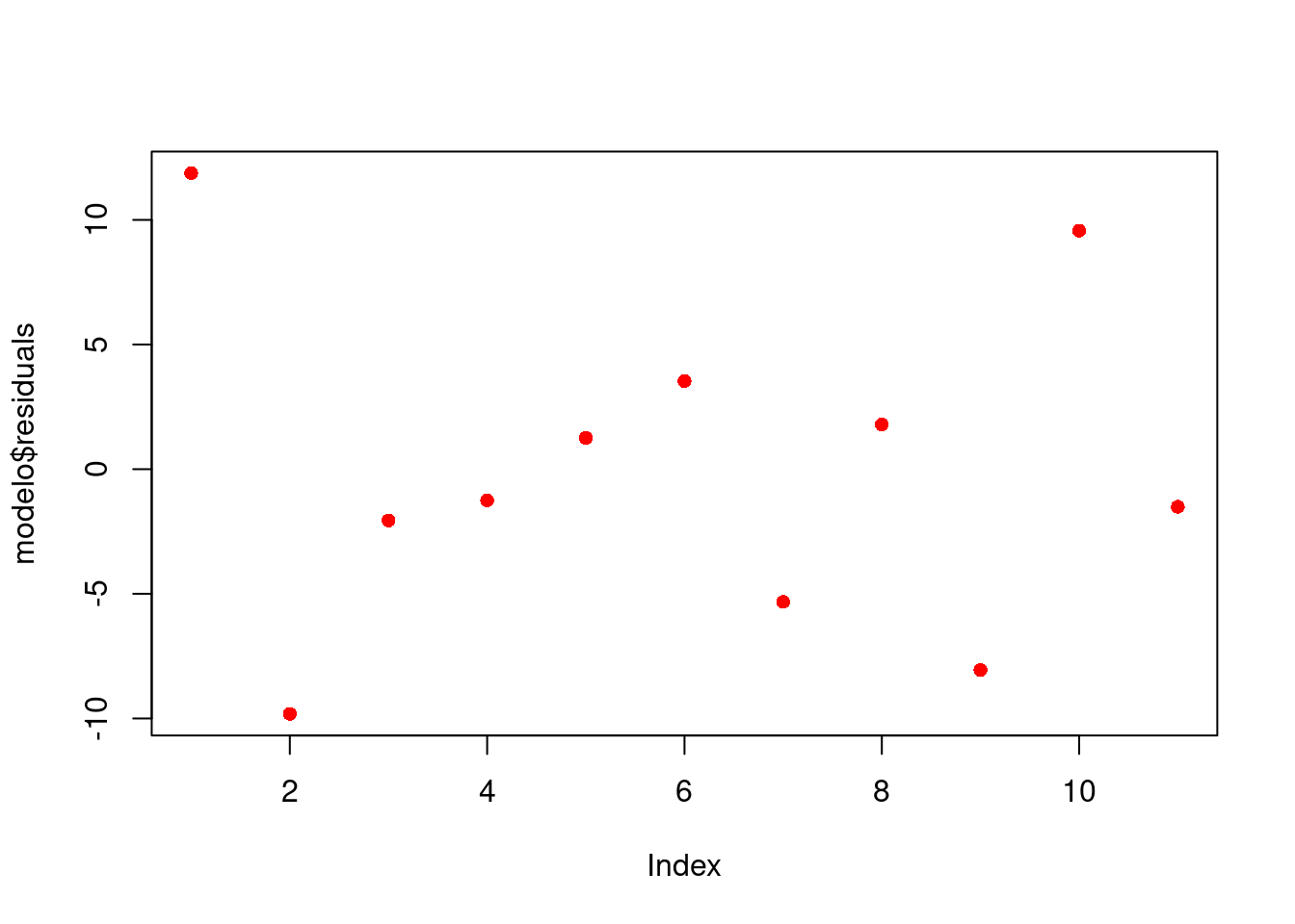
Verificando modelo
library(performance)

check_model(modelo)
2.5.5 Predição
predict(modelo, interval = "prediction")## Warning in predict.lm(modelo, interval = "prediction"): predictions on current data refer to _future_ responses## fit lwr upr
## 1 514.1259 165.2536 862.9982
## 2 576.8163 217.7647 935.8679
## 3 929.0578 549.8593 1308.2563
## 4 545.2501 165.4832 925.0169
## 6 1146.7499 766.9831 1526.5168
## 7 634.4669 257.0284 1011.9055
## 8 767.3224 393.2881 1141.3567
## 9 1147.2107 767.7924 1526.6290
## 10 767.0563 401.0010 1133.1117
## 11 883.4332 523.2959 1243.5705
## 12 1168.5105 788.8965 1548.1245p = predict.lm(modelo, newdata = data.frame(Filhos = as.factor(3), Paes = 386, Vegetais = 608, Frutas = 396, Carnes = 1501, Leite = 319, Alcoolicos = 363))
p## 1
## 501.1353O valor da Ave na linha 5 é 501.135316
Ajustando o conjunto de dados:
# Antes ajuste
dados[5, ]
## # A tibble: 1 × 9
## AreaTrabalho Filhos Paes Vegetais Frutas Carnes Aves Leite Alcoolicos
## <fct> <fct> <dbl> <dbl> <dbl> <dbl> <dbl> <dbl> <dbl>
## 1 EM 3 386 608 396 1501 NA 319 363dados[5, ]['Aves'] = p
# Depois ajuste
dados[5, ]## # A tibble: 1 × 9
## AreaTrabalho Filhos Paes Vegetais Frutas Carnes Aves Leite Alcoolicos
## <fct> <fct> <dbl> <dbl> <dbl> <dbl> <dbl> <dbl> <dbl>
## 1 EM 3 386 608 396 1501 501. 319 3632.5.5.1 Agrupamento
dadosS = subset(dados, select=c("Paes", "Vegetais", "Frutas", "Carnes", "Aves", "Leite", "Alcoolicos"))

d <- dist(dadosS, method = "maximum")
grup = hclust(d, method = "ward.D")
plot(grup, cex = 0.6)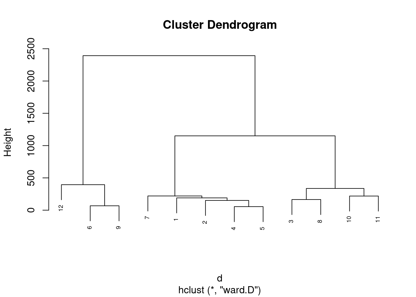
groups <- cutree(grup, k=3)
table(groups, dados$Aves)
##
## groups 501.135316011242 526 544 567 638 759 762 893 927 1148 1149 1167
## 1 1 1 1 1 1 0 0 0 0 0 0 0
## 2 0 0 0 0 0 1 1 1 1 0 0 0
## 3 0 0 0 0 0 0 0 0 0 1 1 1km1 = kmeans(dadosS, 3)
p1 = fviz_cluster(km1, data=dadosS,
palette = c("#2E9FDF", "#FC4E07", "#E7B800", "#E7B700"),
star.plot=FALSE,
# repel=TRUE,
ggtheme=theme_bw())
p1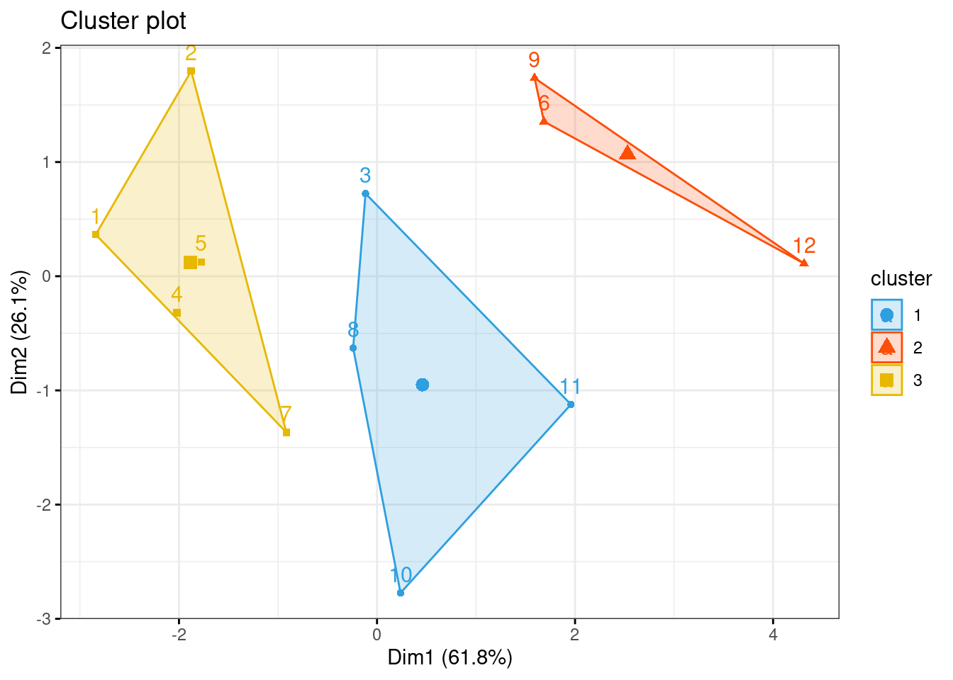
2.5.5.2 Análise Conjunto vendas vs fontes de publicidades
Análise descritiva e regressão linear sobre o conjunto de dados SALES_X_YOUTUBE em DadosAula06.xlsx.
library(readxl)
library(tidyverse)
library(readxl)
library(ggthemes)
library(plotly)
library(knitr)
library(kableExtra)
2.5.5.3 Conjunto de dados
dados03 = read_excel(path = "Dados/04_LABORATORIO REGRESSAO COM DADOS 03_DADOS.xlsx", sheet = 3)
dados03 = dados03[,2:5]
# tail(dados03, 3)

# dados03_t =  pivot_longer(dados03, c(2:5))
# names(dados03_t) = c("Indice", "Grupo", "Valor")
kable(dados03) %>%
  kable_styling(latex_options = "striped")
Vendas em relação aos anúncios no youtube.
## `geom_smooth()` using formula = 'y ~ x'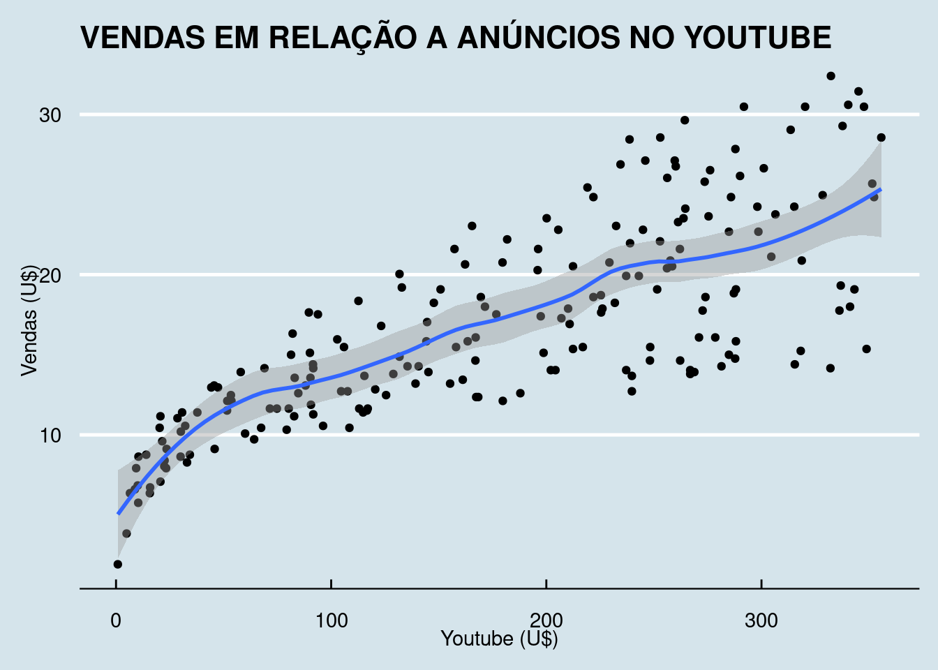
## `geom_smooth()` using formula = 'y ~ x'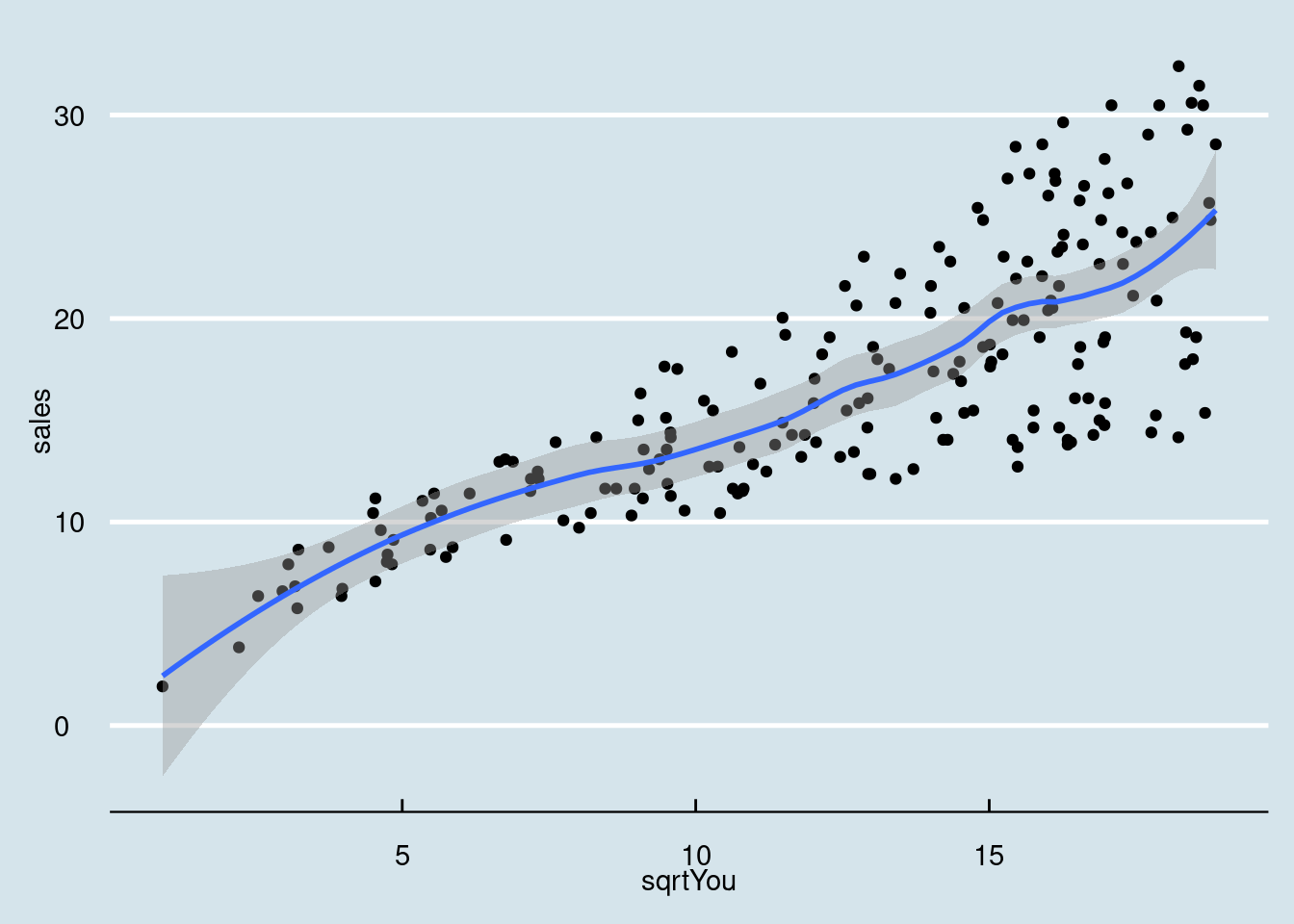
## `geom_smooth()` using formula = 'y ~ x'
Ajustando um modelo linear simples para analise.
model = lm(sales ~ sqrtYou, data = dados03_mod)
summary(model)
##
## Call:
## lm(formula = sales ~ sqrtYou, data = dados03_mod)
##
## Residuals:
## Min 1Q Median 3Q Max
## -8.916 -2.344 -0.131 2.326 9.316
##
## Coefficients:
## Estimate Std. Error t value Pr(>|t|)
## (Intercept) 3.20688 0.80092 4.004 8.8e-05 ***
## sqrtYou 1.09042 0.06029 18.085 < 2e-16 ***
## ---
## Signif. codes: 0 '***' 0.001 '**' 0.01 '*' 0.05 '.' 0.1 ' ' 1
##
## Residual standard error: 3.854 on 198 degrees of freedom
## Multiple R-squared: 0.6229, Adjusted R-squared: 0.621
## F-statistic: 327.1 on 1 and 198 DF, p-value: < 2.2e-16O gráfico mostra observações em relação ao modelo que considero importante para a analise.
plot(sales ~ sqrtYou, data = dados03_mod)
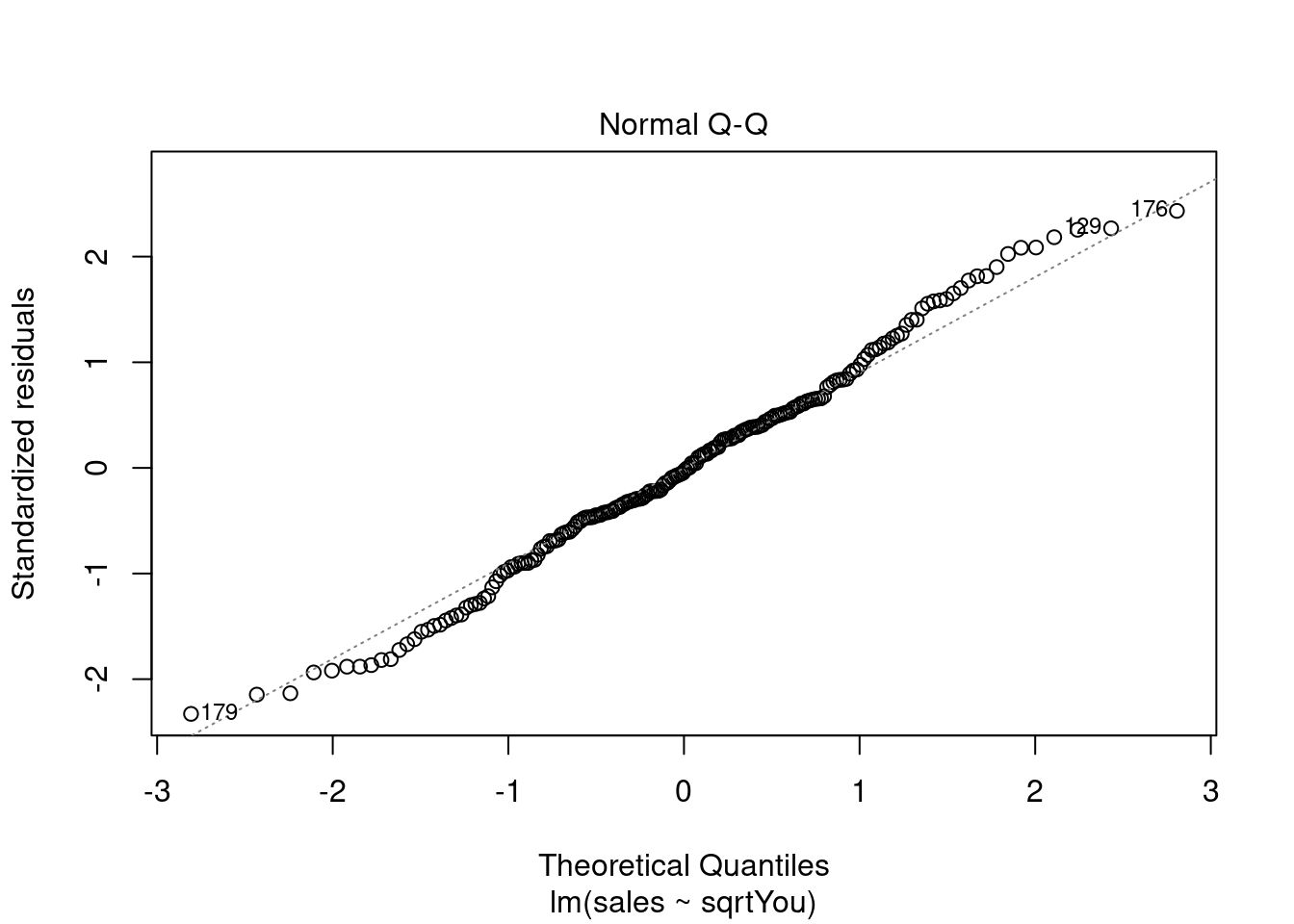
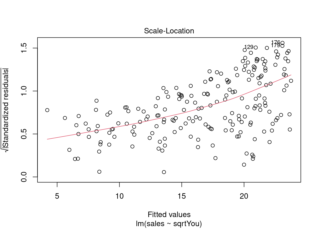
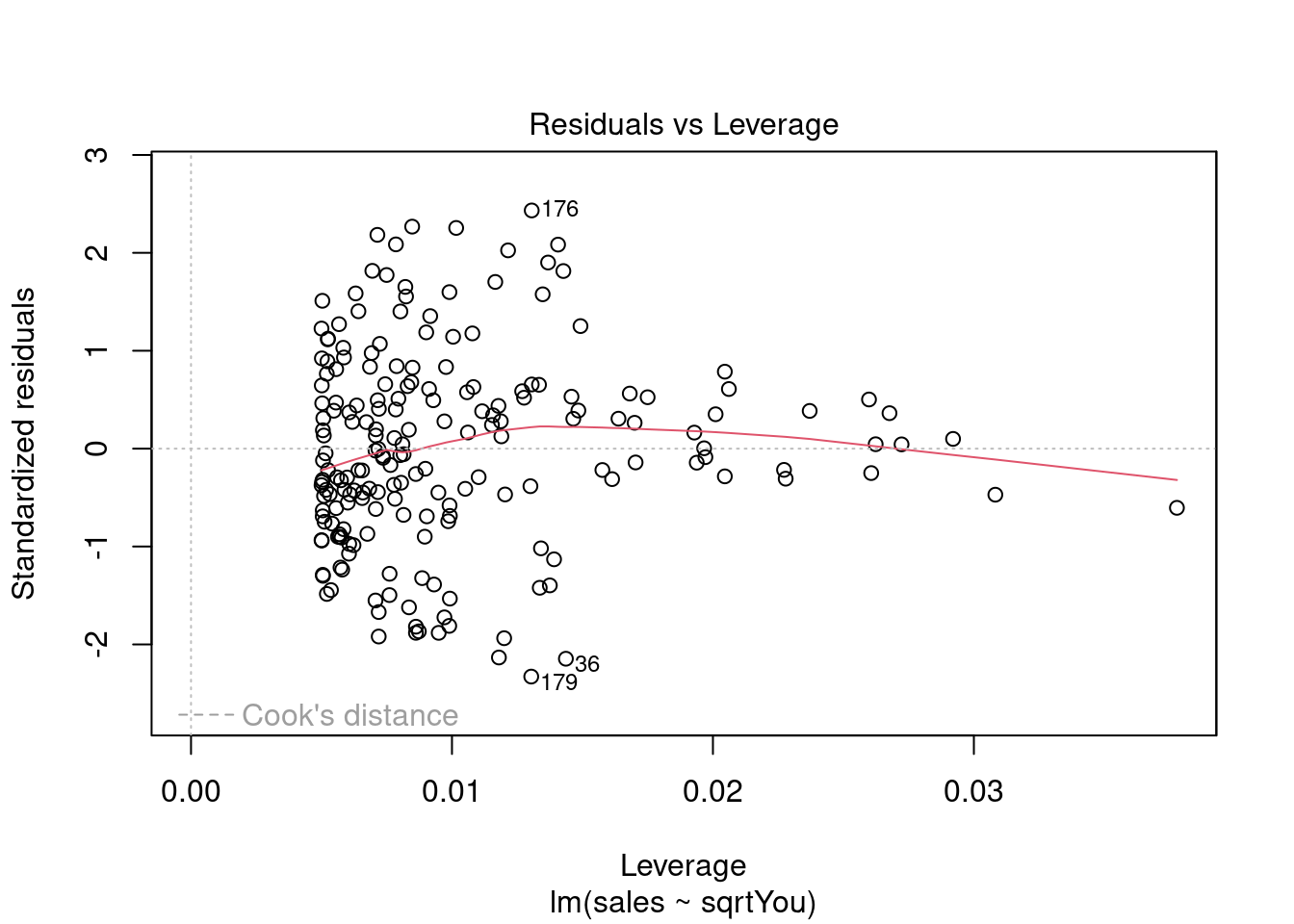
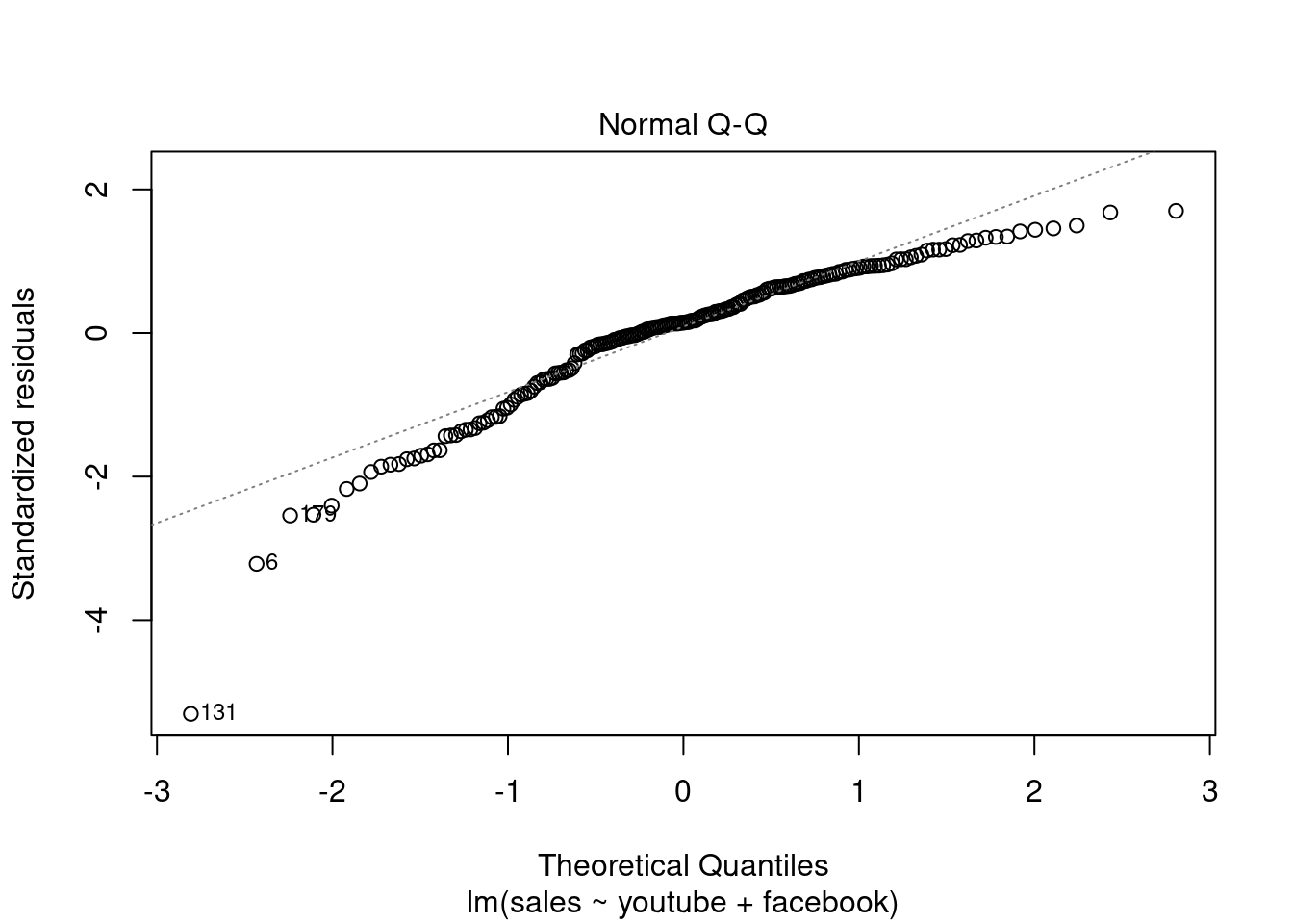
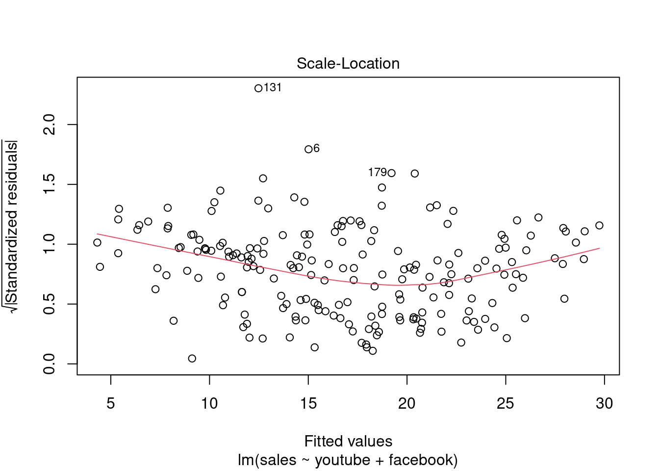
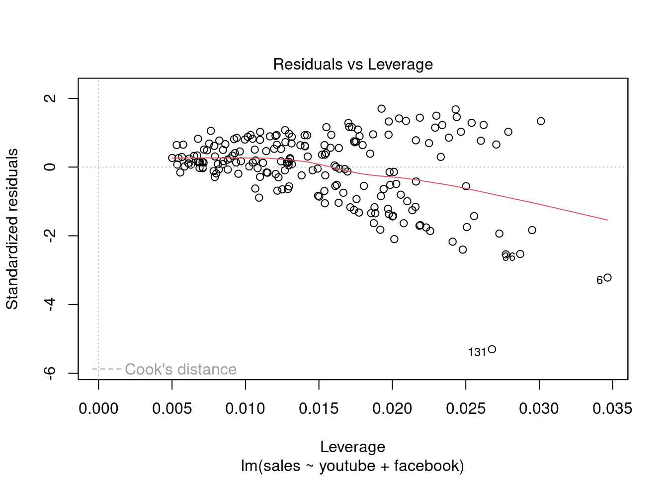
abline(model)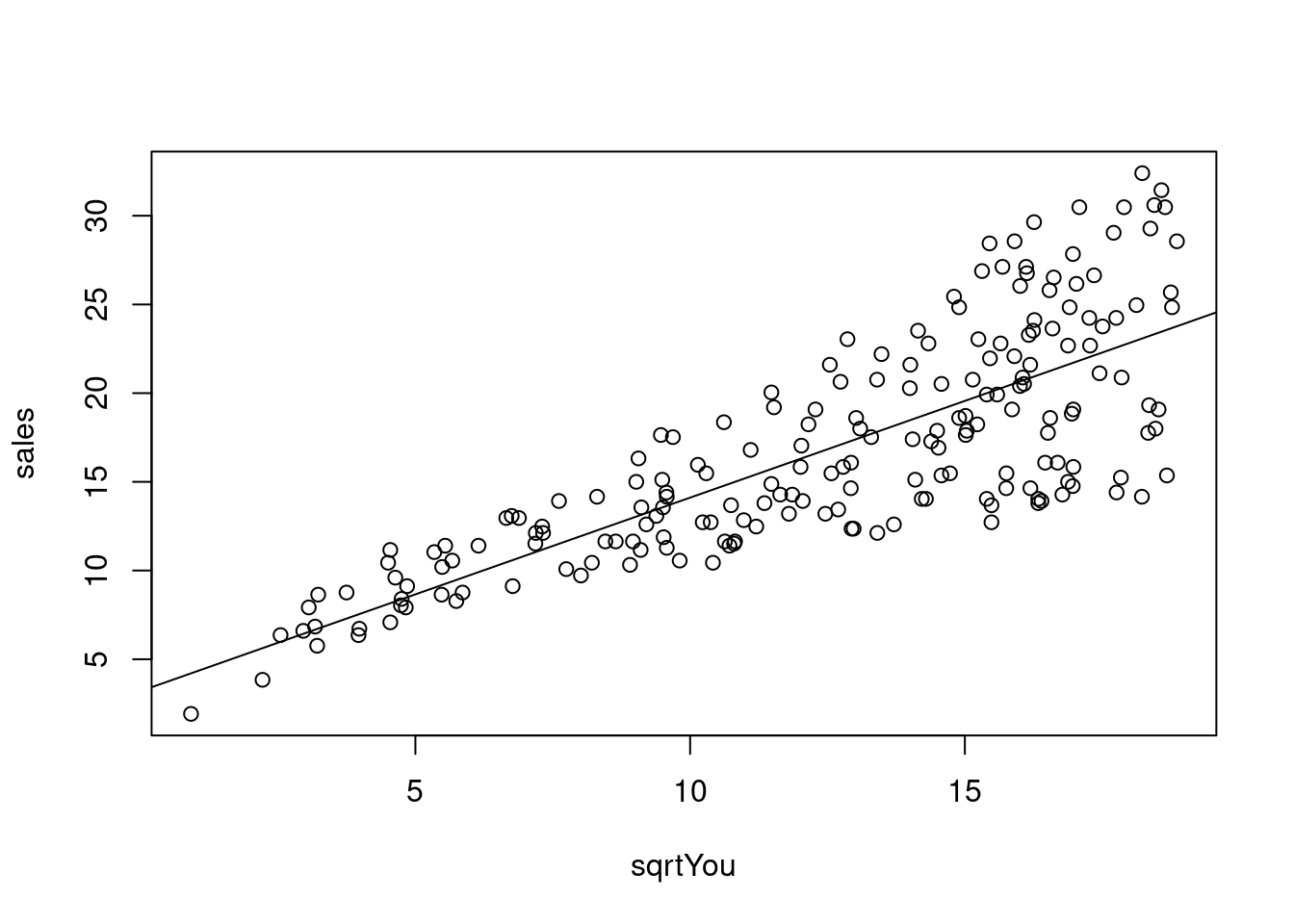 Analisando resíduos.
plot(model)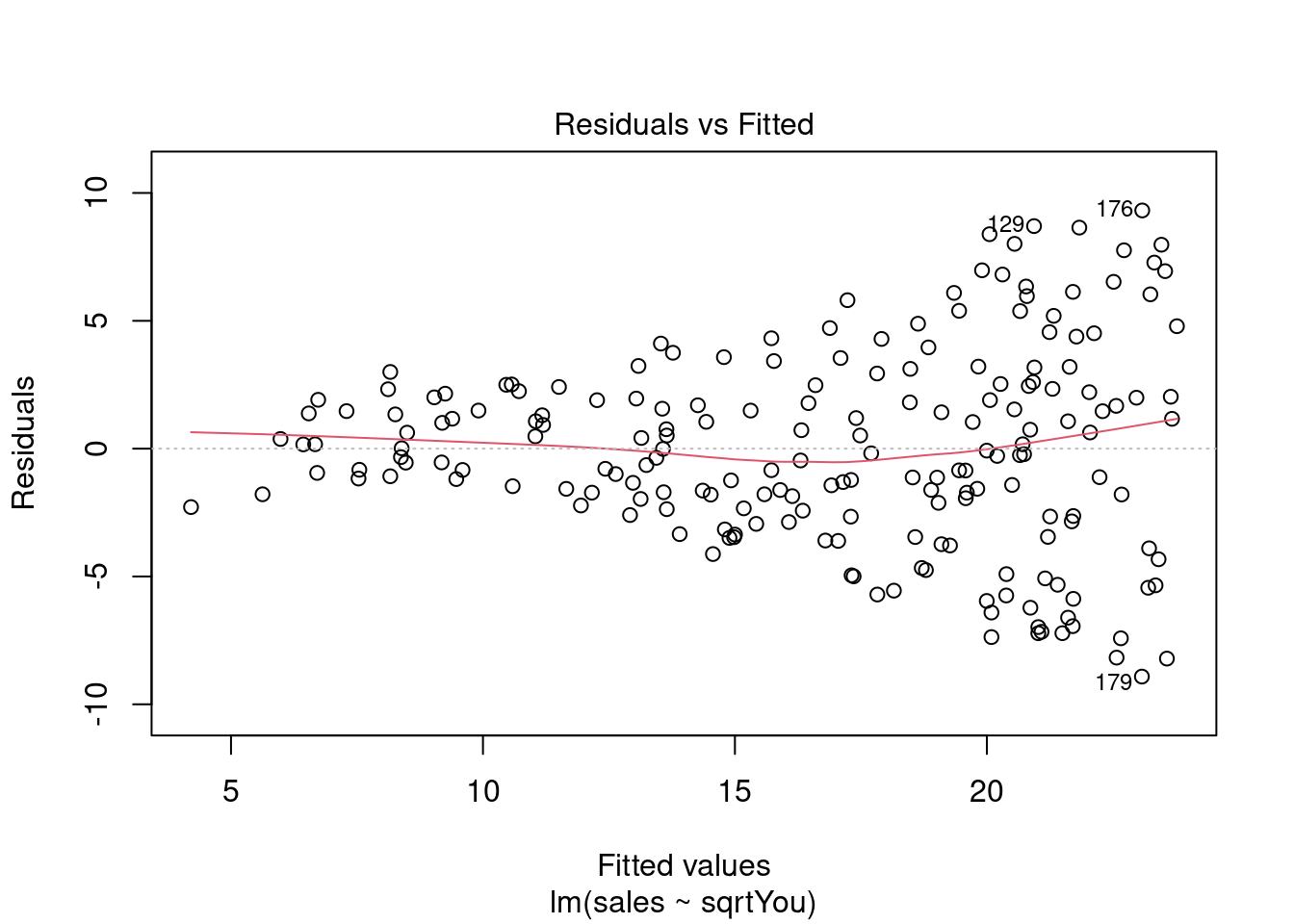
Ajustando o modelo a mais variáveis (multiclass).
modelMult = lm(sales ~ youtube + facebook + newspaper, data = dados03)
summary(modelMult)
##
## Call:
## lm(formula = sales ~ youtube + facebook + newspaper, data = dados03)
##
## Residuals:
## Min 1Q Median 3Q Max
## -10.5932 -1.0690 0.2902 1.4272 3.3951
##
## Coefficients:
## Estimate Std. Error t value Pr(>|t|)
## (Intercept) 3.526667 0.374290 9.422 <2e-16 ***
## youtube 0.045765 0.001395 32.809 <2e-16 ***
## facebook 0.188530 0.008611 21.893 <2e-16 ***
## newspaper -0.001037 0.005871 -0.177 0.86
## ---
## Signif. codes: 0 '***' 0.001 '**' 0.01 '*' 0.05 '.' 0.1 ' ' 1
##
## Residual standard error: 2.023 on 196 degrees of freedom
## Multiple R-squared: 0.8972, Adjusted R-squared: 0.8956
## F-statistic: 570.3 on 3 and 196 DF, p-value: < 2.2e-16plot(modelMult)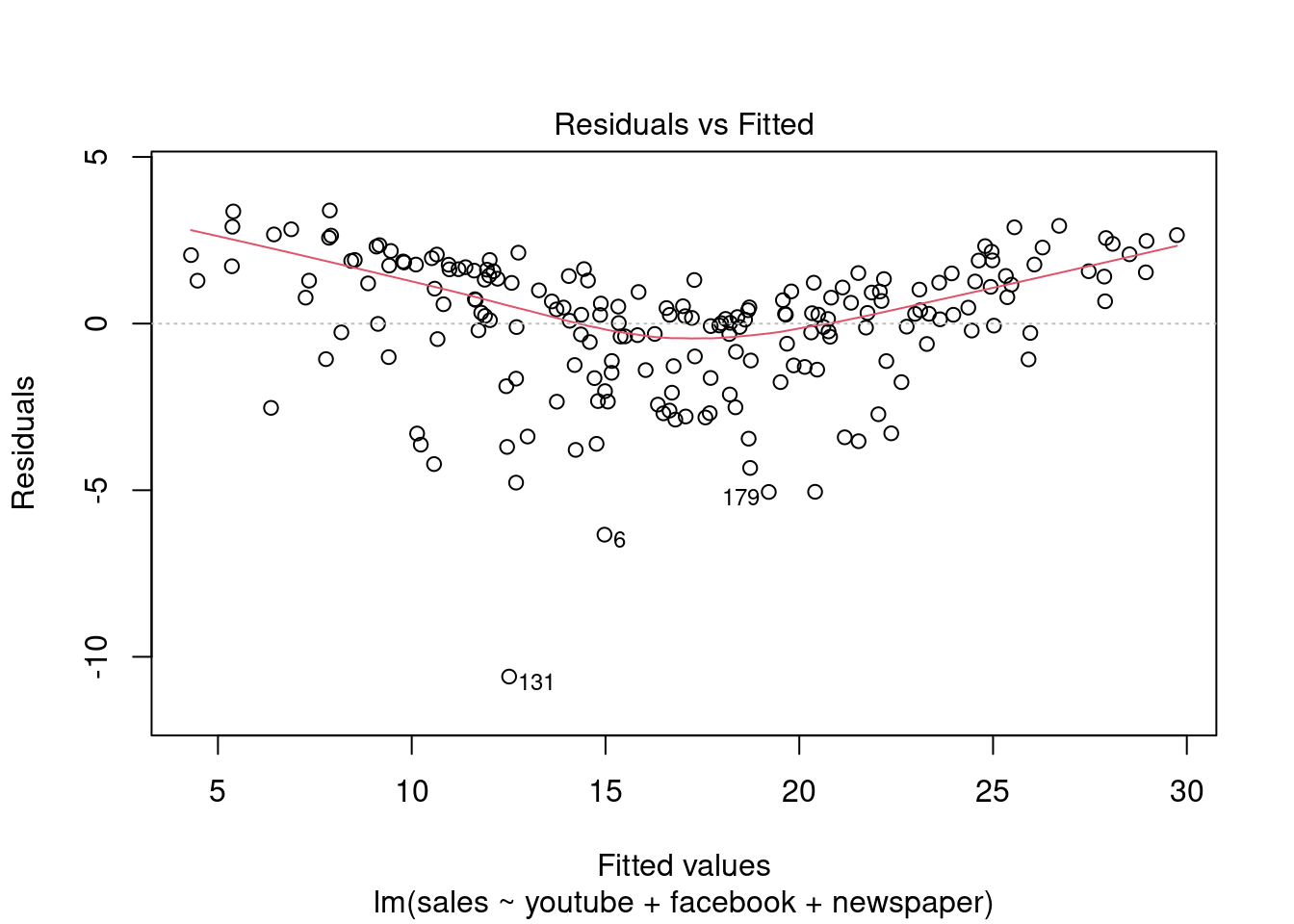
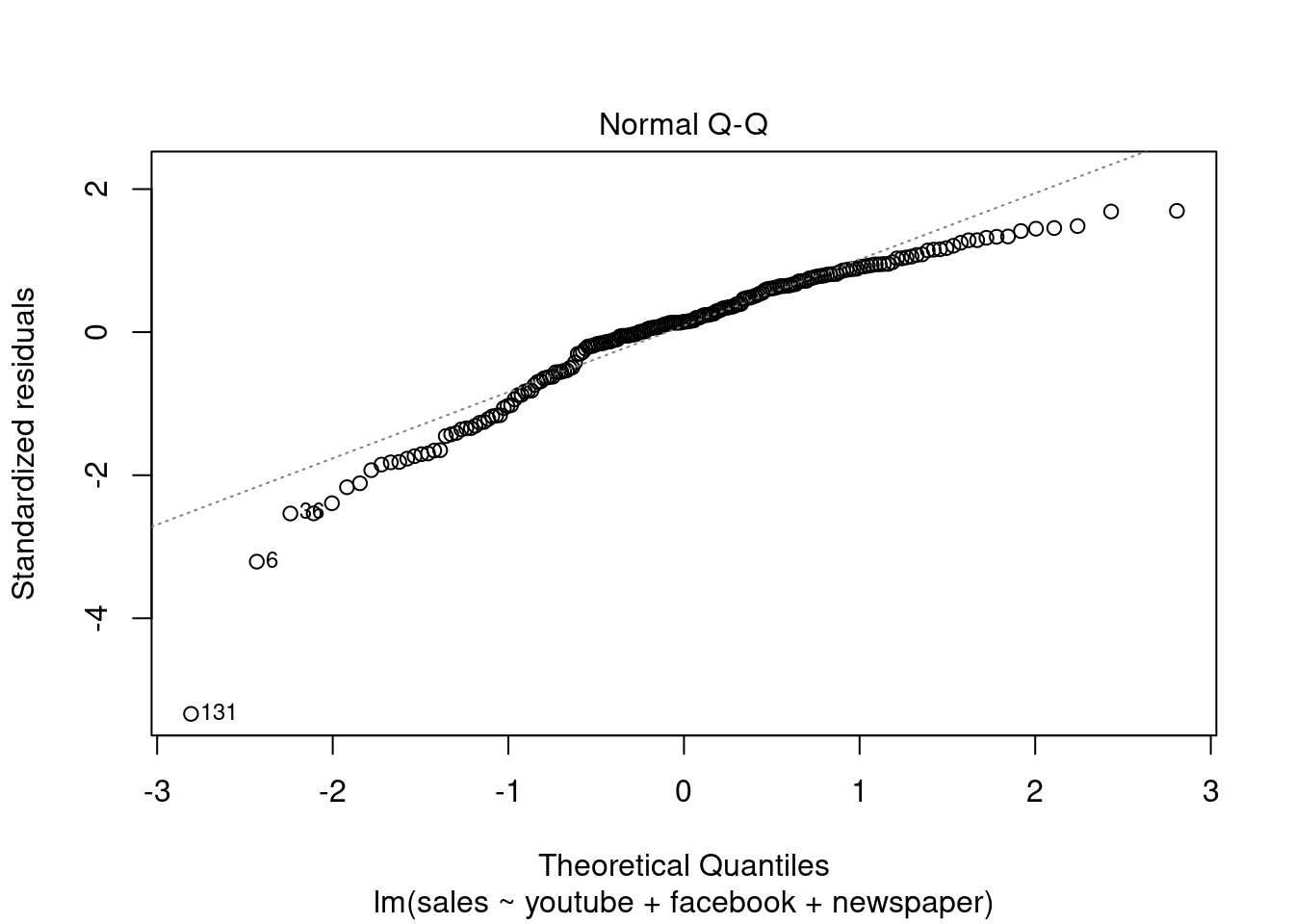
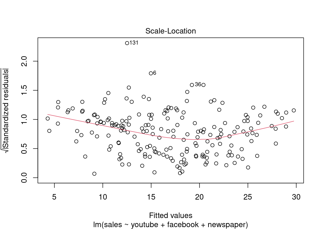
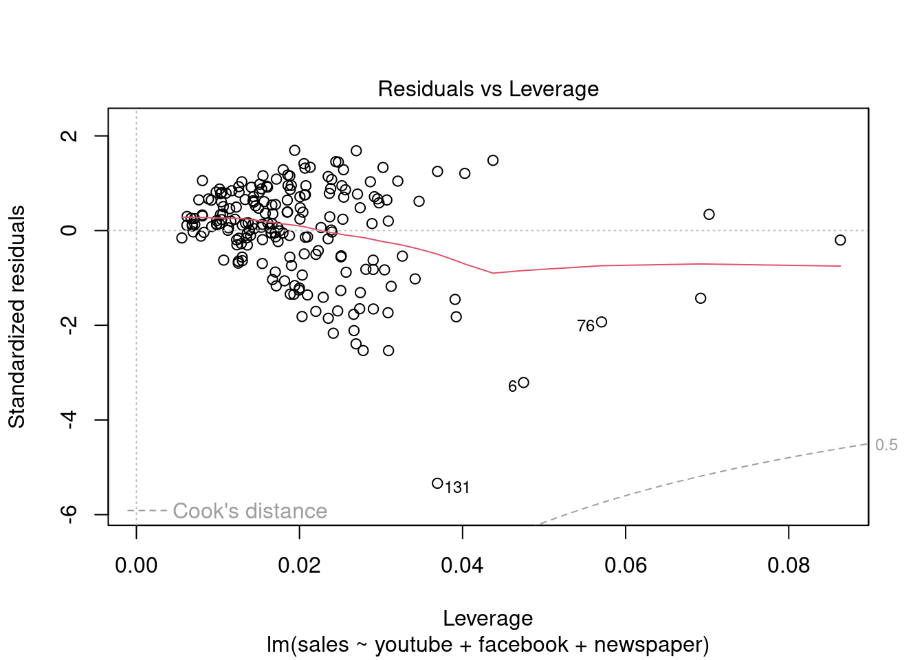
Fica Evidente que o Newspaper tem pouca influência no modelo, sendo o youtube queinfluência nas vendas conforme apresentado.
modelMult2 = lm(sales ~ youtube + facebook, data = dados03)
summary(modelMult2)
##
## Call:
## lm(formula = sales ~ youtube + facebook, data = dados03)
##
## Residuals:
## Min 1Q Median 3Q Max
## -10.5572 -1.0502 0.2906 1.4049 3.3994
##
## Coefficients:
## Estimate Std. Error t value Pr(>|t|)
## (Intercept) 3.50532 0.35339 9.919 <2e-16 ***
## youtube 0.04575 0.00139 32.909 <2e-16 ***
## facebook 0.18799 0.00804 23.382 <2e-16 ***
## ---
## Signif. codes: 0 '***' 0.001 '**' 0.01 '*' 0.05 '.' 0.1 ' ' 1
##
## Residual standard error: 2.018 on 197 degrees of freedom
## Multiple R-squared: 0.8972, Adjusted R-squared: 0.8962
## F-statistic: 859.6 on 2 and 197 DF, p-value: < 2.2e-16plot(modelMult2)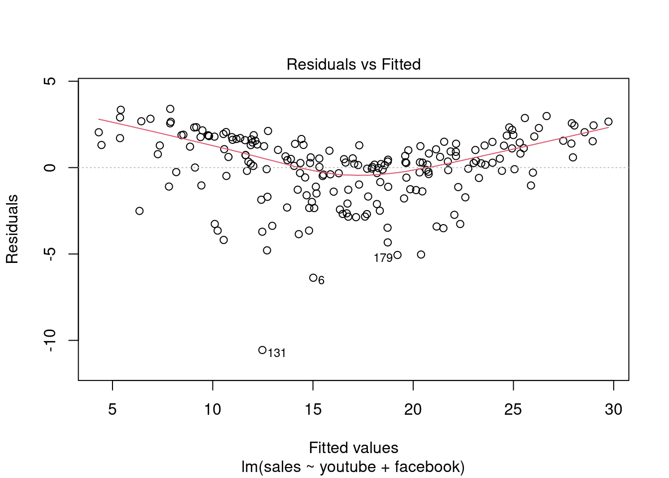
2.5.5.4 Pacotes
Pacotes carregados apos serem instalados para estes exercícios:
library(readxl)
library(tidyverse)
library(readxl)
library(ggthemes)
library(plotly)
library(knitr)
library(kableExtra)
2.5.5.4.1 Conjunto de dados
Analise se o cliente pode receber o crédito de acordo com a análise. As variáveis são:
- ST - Situação (0 - Passou na análise, 1 - Nâo passou na análise) - Y
- R - Renda - X
- ND - Num Dependentes - X
- VE - Vinculo Empregaticio - X
dados04 = read_excel(path = "Dados/04_LABORATORIO REGRESSAO COM DADOS 03_DADOS.xlsx", sheet = 4)
dados04 = dados04[,18:21]
dados04$ST = factor(dados04$ST)
dados04$VE = factor(dados04$VE)

kable(dados04) %>%
  kable_styling(latex_options = "striped")
Situação explicada pela renda.
plot(dados04$R ~ dados04$ST)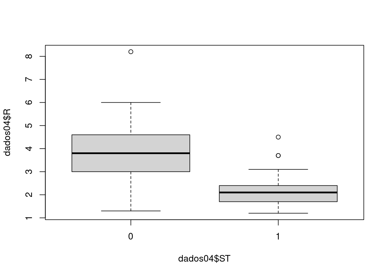
# table(dados04$VE, dados04$ST)O modelo é
\[ \log{\left(\frac{P(y_i=1)}{1-P(y_i=1)}\right)} = \beta_0 + \beta_1 x_1 + \beta_2 x_2 + \beta_3 x_3 + \epsilon_i \]
\[ \frac{P(y=1)}{1-P(y=1)} = e^{(\beta_0 + \beta_1 x_1 + \beta_2 x_2 + \beta_3 x_3)} \]
O ajuste é
modelo04  = glm(dados04$ST ~ dados04$R + dados04$ND + dados04$VE, family = binomial(link='logit'))
valoresPredito = predict.glm(modelo04, type = "response")
summary(modelo04)
##
## Call:
## glm(formula = dados04$ST ~ dados04$R + dados04$ND + dados04$VE,
## family = binomial(link = "logit"))
##
## Deviance Residuals:
## Min 1Q Median 3Q Max
## -2.6591 -0.2633 -0.0531 0.4187 2.0147
##
## Coefficients:
## Estimate Std. Error z value Pr(>|z|)
## (Intercept) 1.1117 1.5725 0.707 0.479578
## dados04$R -1.7872 0.4606 -3.880 0.000105 ***
## dados04$ND 0.9031 0.3857 2.341 0.019212 *
## dados04$VE1 2.9113 0.8506 3.423 0.000620 ***
## ---
## Signif. codes: 0 '***' 0.001 '**' 0.01 '*' 0.05 '.' 0.1 ' ' 1
##
## (Dispersion parameter for binomial family taken to be 1)
##
## Null deviance: 126.450 on 91 degrees of freedom
## Residual deviance: 51.382 on 88 degrees of freedom
## AIC: 59.382
##
## Number of Fisher Scoring iterations: 6Os valores preditos são:
## Warning in confusionMatrix.default(valoresPredito_cl, dados04$ST): Levels are not in the same order for reference
## and data. Refactoring data to match.

## Warning in confusionMatrix.default(valoresPredito_cl, dados04$ST): Levels are not in the same order for reference
## and data. Refactoring data to match.
## Confusion Matrix and Statistics
##
## Reference
## Prediction 0 1
## 0 46 5
## 1 5 36
##
## Accuracy : 0.8913
## 95% CI : (0.8092, 0.9466)
## No Information Rate : 0.5543
## P-Value [Acc > NIR] : 2.554e-12
##
## Kappa : 0.78
##
## Mcnemar's Test P-Value : 1
##
## Sensitivity : 0.9020
## Specificity : 0.8780
## Pos Pred Value : 0.9020
## Neg Pred Value : 0.8780
## Prevalence : 0.5543
## Detection Rate : 0.5000
## Detection Prevalence : 0.5543
## Balanced Accuracy : 0.8900
##
## 'Positive' Class : 0
## Matriz de confusão
draw_confusion_matrix(cm)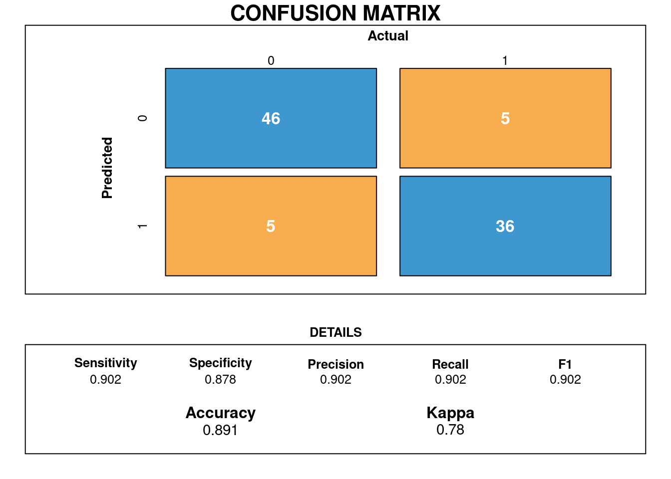
Podemos assumir que a acurácia do modelo é de 89% com sensibilidade em torno de 90%. Foi Possivel treinar os dados o que resultou em um bom acerto de 100% (46/46). No que se refere a especificidade é de 88% havendo confusão com 5/46 observações. O mesmo ocorreu para quando nao ocorreu bom acerto que foi 36/46 observações onde estão corretas e 5/46 não estao.
2.5.5.4.2 Classificação de tipos faciais
Os dados do arquivo tipofacialforam extraídos de um estudo odontológico realizado pelo Dr. Flávio Cotrim Vellini. Um dos objetivos era utilizar medidas entre diferentes pontos do crânio para caracterizar indivíduos com diferentes tipos faciais, a saber, braquicéfalos, mesocéfalos e dolicocéfalos (grupos). O conjunto de dados contém observações de 11 variáveis em 101 pacientes. Para efeitos didáticos, considere apenas a altura facial (altfac) e a profundidade facial (proffac) como variáveis preditoras.
2.5.5.6 Conjunto de dados
httr::GET("http://www.ime.usp.br/~jmsinger/MorettinSinger/tipofacial.xls", httr::write_disk("Dados/tipofacial.xls", overwrite = TRUE))## Response [https://www.ime.usp.br/~jmsinger/MorettinSinger/tipofacial.xls]
## Date: 2022-12-13 23:42
## Status: 200
## Content-Type: application/vnd.ms-excel
## Size: 20.5 kB
## <ON DISK> /home/emau/R/Caderno_Eder/BIG019_Eder/Dados/tipofacial.xlstipofacial <- read_excel("Dados/tipofacial.xls")
str(tipofacial)## tibble [101 × 13] (S3: tbl_df/tbl/data.frame)
## $ paciente: num [1:101] 10 10 27 39 39 39 55 76 77 133 ...
## $ sexo : chr [1:101] "M" "M" "F" "F" ...
## $ grupo : chr [1:101] "braq" "braq" "braq" "braq" ...
## $ idade : num [1:101] 5.58 11.42 16.17 4.92 10.92 ...
## $ nsba : num [1:101] 132 134 122 130 130 ...
## $ ns : num [1:101] 58 63 77.5 64 70 68.5 71 72 70 80 ...
## $ sba : num [1:101] 36 42.5 48 34.5 36.5 41.5 42 46.5 44 52 ...
## $ altfac : num [1:101] 1.2 1.2 2.6 3.1 3.1 3.3 2.4 1.9 2.1 2.8 ...
## $ proffac : num [1:101] 0.8 0.4 0.2 -1 0.6 -0.6 0.3 0.5 -0.1 0.2 ...
## $ eixofac : num [1:101] 0.4 1 0.3 1.9 1.2 1.1 1.1 1.4 2.2 0.4 ...
## $ planmand: num [1:101] 0.4 1 0.9 1.3 2.2 1.2 1.2 0.6 0.8 1.1 ...
## $ arcomand: num [1:101] 2.5 3.6 3.4 1.6 2.3 2.1 3.5 3.5 0.7 1.8 ...
## $ vert : num [1:101] 1.06 1.44 1.48 1.38 1.88 1.42 1.7 1.58 1.14 1.26 ...Número de observações 101.
2.5.5.7 Categorizando as variaveis de grupo.
# Considerar (altfac) e a profundidade facial (proffac) como variáveis preditoras.

tipofacial$sumfac = tipofacial$altfac + tipofacial$proffac
tipofacial$grupo = as.factor(tipofacial$grupo)plot(tipofacial$sumfac ~ tipofacial$grupo)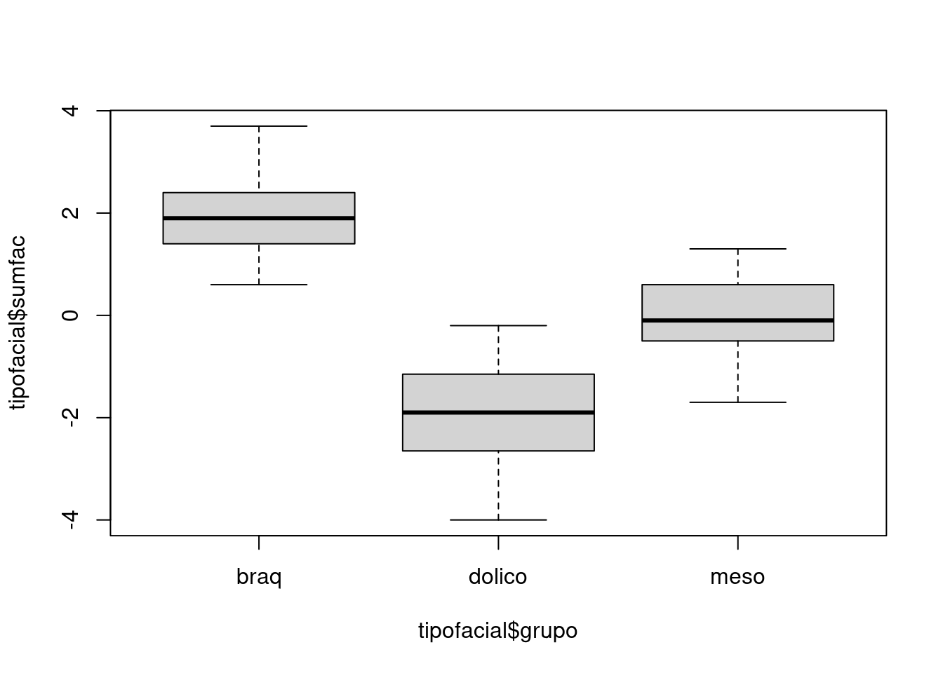
print(tipofacial, n = 32)## # A tibble: 101 × 14
## paciente sexo grupo idade nsba ns sba altfac proffac eixofac planmand arcomand vert sumfac
## <dbl> <chr> <fct> <dbl> <dbl> <dbl> <dbl> <dbl> <dbl> <dbl> <dbl> <dbl> <dbl> <dbl>
## 1 10 M braq 5.58 132 58 36 1.2 0.8 0.4 0.4 2.5 1.06 2
## 2 10 M braq 11.4 134 63 42.5 1.2 0.4 1 1 3.6 1.44 1.6
## 3 27 F braq 16.2 122. 77.5 48 2.6 0.2 0.3 0.9 3.4 1.48 2.8
## 4 39 F braq 4.92 130. 64 34.5 3.1 -1 1.9 1.3 1.6 1.38 2.1
## 5 39 F braq 10.9 130. 70 36.5 3.1 0.6 1.2 2.2 2.3 1.88 3.7
## 6 39 F braq 12.9 128 68.5 41.5 3.3 -0.6 1.1 1.2 2.1 1.42 2.7
## 7 55 F braq 16.8 130 71 42 2.4 0.3 1.1 1.2 3.5 1.7 2.7
## 8 76 F braq 16 125 72 46.5 1.9 0.5 1.4 0.6 3.5 1.58 2.4
## 9 77 F braq 17.1 130. 70 44 2.1 -0.1 2.2 0.8 0.7 1.14 2
## 10 133 M braq 14.8 130 80 52 2.8 0.2 0.4 1.1 1.8 1.26 3
## 11 145 F braq 10.7 118. 67 43.5 1.2 0.7 1.7 1.5 0.9 1.2 1.9
## 12 148 F braq 11.3 129 68 41.5 2.9 -0.7 2.2 1.3 2.2 1.58 2.2
## 13 165 F braq 15 137 74 43 2.1 -0.3 1.3 1.2 2.5 1.36 1.8
## 14 176 M braq 5.67 134 65 39 2.5 0.2 2.1 2.2 3.1 2.02 2.7
## 15 176 M braq 13 130 72 48 2.2 0.2 2.9 2.4 4 2.34 2.4
## 16 208 M braq 13.8 130 67.5 43 0.9 1.5 -0.4 1.2 2.3 1.1 2.4
## 17 246 F braq 11.8 129 67 43 0.8 1.1 1.5 0.3 1.4 1.02 1.9
## 18 27 F braq 4.67 126 63 35 1.9 0.2 0.3 0.1 1.6 0.82 2.1
## 19 39 F braq 3.67 131 61 32 3 -1.4 1.8 0.7 0.8 0.98 1.6
## 20 45 M braq 22.7 133 77 46 1.7 -0.9 -0.6 0.3 2.7 0.64 0.8
## 21 49 F braq 16.6 136. 71 42 1 0.5 0.1 0.2 2.7 0.9 1.5
## 22 52 M braq 12.6 126. 69 41.5 1.4 0 0.4 0.5 2.5 0.96 1.4
## 23 63 F braq 6.17 130. 63 37 1.9 -0.5 0.8 0.5 1.3 0.8 1.4
## 24 63 F braq 15.7 132 72.5 43 1.9 0 2 0.4 0.3 0.92 1.9
## 25 68 M braq 13.8 128 72 43 1.2 -0.6 1 1.1 2.3 1 0.6
## 26 76 F braq 5.33 124 61 39.5 1.3 -0.3 -0.1 0.6 1.6 0.62 1
## 27 86 F braq 5.25 126. 61.5 42.5 1.1 0 -0.1 0.2 2.7 0.78 1.1
## 28 109 M braq 14.9 131 78.5 50 1.8 -0.4 1.1 0.8 1.3 0.92 1.4
## 29 145 F braq 3.67 129 60 37.5 1 0 1.1 0.1 0.4 0.52 1
## 30 148 F braq 4.25 127 61.5 34 1.9 0.2 1.6 0 1.4 1.02 2.1
## 31 155 F braq 5.25 127 65 39.5 1.2 -0.5 1.2 0.2 1.4 0.7 0.7
## 32 155 F braq 11.3 128 71.5 45 2.3 -0.3 0.7 0.4 2.2 0.8 2
## # … with 69 more rowssummary(tipofacial)## paciente sexo grupo idade nsba ns sba
## Min. : 10.0 Length:101 braq :33 Min. : 3.670 Min. :117.0 Min. :57.00 Min. :32.0
## 1st Qu.: 61.0 Class :character dolico:31 1st Qu.: 5.250 1st Qu.:125.0 1st Qu.:63.00 1st Qu.:38.5
## Median :105.0 Mode :character meso :37 Median :10.000 Median :128.0 Median :66.50 Median :41.5
## Mean :108.4 Mean : 9.204 Mean :127.7 Mean :67.03 Mean :41.5
## 3rd Qu.:148.0 3rd Qu.:12.580 3rd Qu.:130.0 3rd Qu.:71.00 3rd Qu.:44.0
## Max. :246.0 Max. :22.670 Max. :137.0 Max. :81.00 Max. :54.0
## altfac proffac eixofac planmand arcomand vert
## Min. :-2.3000 Min. :-2.7000 Min. :-3.5000 Min. :-2.9000 Min. :-2.3000 Min. :-1.92000
## 1st Qu.:-0.3000 1st Qu.:-1.2000 1st Qu.:-1.0000 1st Qu.:-1.3000 1st Qu.: 0.0000 1st Qu.:-0.68000
## Median : 0.6000 Median :-0.7000 Median :-0.2000 Median :-0.5000 Median : 0.8000 Median : 0.00000
## Mean : 0.6238 Mean :-0.6119 Mean :-0.1129 Mean :-0.4693 Mean : 0.8386 Mean : 0.04931
## 3rd Qu.: 1.7000 3rd Qu.: 0.0000 3rd Qu.: 0.8000 3rd Qu.: 0.4000 3rd Qu.: 1.6000 3rd Qu.: 0.80000
## Max. : 3.3000 Max. : 1.5000 Max. : 2.9000 Max. : 2.4000 Max. : 4.0000 Max. : 2.34000
## sumfac
## Min. :-4.00000
## 1st Qu.:-0.90000
## Median :-0.10000
## Mean : 0.01188
## 3rd Qu.: 1.40000
## Max. : 3.70000sd(tipofacial$sumfac)## [1] 1.750331Dataframe para comparar as métricas dos modelos.
model_eval <- data.frame(matrix(ncol = 9, nrow = 0))

colnames(model_eval) <- c('Model', 'Algorithm', 'Accuracy', 'Sensitivity_C1', 'Sensitivity_C2', 'Sensitivity_C3', 'Specificity_C1', 'Specificity_C2', 'Specificity_C3')
2.5.5.8 Generalizando os Modelos Lineares
glm.fit = multinom(grupo ~ sumfac, data=tipofacial)## # weights: 9 (4 variable)
## initial value 110.959841
## iter 10 value 38.508219
## final value 38.456349
## convergedsummary(glm.fit)## Call:
## multinom(formula = grupo ~ sumfac, data = tipofacial)
##
## Coefficients:
## (Intercept) sumfac
## dolico 1.532730 -6.173138
## meso 3.781329 -3.762457
##
## Std. Errors:
## (Intercept) sumfac
## dolico 1.238970 1.174600
## meso 1.107069 1.005516
##
## Residual Deviance: 76.9127
## AIC: 84.9127predito = predict(glm.fit, newdata = tipofacial)
cm = confusionMatrix(predito, tipofacial$grupo)
cm## Confusion Matrix and Statistics
##
## Reference
## Prediction braq dolico meso
## braq 27 0 4
## dolico 0 23 2
## meso 6 8 31
##
## Overall Statistics
##
## Accuracy : 0.802
## 95% CI : (0.7109, 0.8746)
## No Information Rate : 0.3663
## P-Value [Acc > NIR] : < 2.2e-16
##
## Kappa : 0.7002
##
## Mcnemar's Test P-Value : NA
##
## Statistics by Class:
##
## Class: braq Class: dolico Class: meso
## Sensitivity 0.8182 0.7419 0.8378
## Specificity 0.9412 0.9714 0.7812
## Pos Pred Value 0.8710 0.9200 0.6889
## Neg Pred Value 0.9143 0.8947 0.8929
## Prevalence 0.3267 0.3069 0.3663
## Detection Rate 0.2673 0.2277 0.3069
## Detection Prevalence 0.3069 0.2475 0.4455
## Balanced Accuracy 0.8797 0.8567 0.8095# Adiciona as métricas no df
model_eval[nrow(model_eval) + 1,] <- c("glm.fit", "glm", cm$overall['Accuracy'], cm$byClass[,1], cm$byClass[,2])Dividindo os dados de treinamento em uma faixa de (70%) e os dados de testes em (30%).
alpha=0.7
d = sort(sample(nrow(tipofacial), nrow(tipofacial)*alpha))
train = tipofacial[d,]
test = tipofacial[-d,]

glm.fit = multinom(grupo ~ sumfac, data=train)
## # weights: 9 (4 variable)
## initial value 76.902860
## iter 10 value 25.631167
## final value 25.471240
## convergedsummary(glm.fit)## Call:
## multinom(formula = grupo ~ sumfac, data = train)
##
## Coefficients:
## (Intercept) sumfac
## dolico 1.908414 -6.890985
## meso 3.863119 -4.681112
##
## Std. Errors:
## (Intercept) sumfac
## dolico 1.686495 1.804328
## meso 1.562814 1.671748
##
## Residual Deviance: 50.94248
## AIC: 58.94248predito = predict(glm.fit, newdata = test)
cm = confusionMatrix(predito, test$grupo)
cm## Confusion Matrix and Statistics
##
## Reference
## Prediction braq dolico meso
## braq 7 0 4
## dolico 0 5 1
## meso 1 2 11
##
## Overall Statistics
##
## Accuracy : 0.7419
## 95% CI : (0.5539, 0.8814)
## No Information Rate : 0.5161
## P-Value [Acc > NIR] : 0.008762
##
## Kappa : 0.5914
##
## Mcnemar's Test P-Value : NA
##
## Statistics by Class:
##
## Class: braq Class: dolico Class: meso
## Sensitivity 0.8750 0.7143 0.6875
## Specificity 0.8261 0.9583 0.8000
## Pos Pred Value 0.6364 0.8333 0.7857
## Neg Pred Value 0.9500 0.9200 0.7059
## Prevalence 0.2581 0.2258 0.5161
## Detection Rate 0.2258 0.1613 0.3548
## Detection Prevalence 0.3548 0.1935 0.4516
## Balanced Accuracy 0.8505 0.8363 0.7438# Adiciona as métricas no df
model_eval[nrow(model_eval) + 1,] <- c("glm.fit-split", "glm", cm$overall['Accuracy'], cm$byClass[,1], cm$byClass[,2])kable(model_eval) %>%
kable_styling(latex_options = "striped")| Model | Algorithm | Accuracy | Sensitivity_C1 | Sensitivity_C2 | Sensitivity_C3 | Specificity_C1 | Specificity_C2 | Specificity_C3 |
|---|---|---|---|---|---|---|---|---|
| glm.fit | glm | 0.801980198019802 | 0.818181818181818 | 0.741935483870968 | 0.837837837837838 | 0.941176470588235 | 0.971428571428571 | 0.78125 |
| glm.fit-split | glm | 0.741935483870968 | 0.875 | 0.714285714285714 | 0.6875 | 0.826086956521739 | 0.958333333333333 | 0.8 |
Treinar o modelo com dados diferentes em um grupo mostrou que o modelo tem uma capacidade de assertividade e tambem generalizar as infos apresentadas.
2.5.5.9 Analise Descr. Linear - Fisher
modFisher01 = lda(grupo ~ sumfac, data = tipofacial)
predito = predict(modFisher01)
classPred = predito$class
cm = confusionMatrix(classPred, tipofacial$grupo)
cm
## Confusion Matrix and Statistics
##
## Reference
## Prediction braq dolico meso
## braq 29 0 5
## dolico 0 23 2
## meso 4 8 30
##
## Overall Statistics
##
## Accuracy : 0.8119
## 95% CI : (0.7219, 0.8828)
## No Information Rate : 0.3663
## P-Value [Acc > NIR] : < 2.2e-16
##
## Kappa : 0.7157
##
## Mcnemar's Test P-Value : NA
##
## Statistics by Class:
##
## Class: braq Class: dolico Class: meso
## Sensitivity 0.8788 0.7419 0.8108
## Specificity 0.9265 0.9714 0.8125
## Pos Pred Value 0.8529 0.9200 0.7143
## Neg Pred Value 0.9403 0.8947 0.8814
## Prevalence 0.3267 0.3069 0.3663
## Detection Rate 0.2871 0.2277 0.2970
## Detection Prevalence 0.3366 0.2475 0.4158
## Balanced Accuracy 0.9026 0.8567 0.8117# Adiciona as métricas no df
model_eval[nrow(model_eval) + 1,] <- c("modFisher01", "lda", cm$overall['Accuracy'], cm$byClass[,1], cm$byClass[,2])2.5.5.10 Bayes
modBayes01 = lda(grupo ~ sumfac, data = tipofacial, prior = c(0.25, 0.50, 0.25))
predito = predict(modBayes01)
classPred = predito$class
cm = confusionMatrix(classPred, tipofacial$grupo)
cm
## Confusion Matrix and Statistics
##
## Reference
## Prediction braq dolico meso
## braq 29 0 5
## dolico 0 24 6
## meso 4 7 26
##
## Overall Statistics
##
## Accuracy : 0.7822
## 95% CI : (0.689, 0.8582)
## No Information Rate : 0.3663
## P-Value [Acc > NIR] : < 2.2e-16
##
## Kappa : 0.6723
##
## Mcnemar's Test P-Value : NA
##
## Statistics by Class:
##
## Class: braq Class: dolico Class: meso
## Sensitivity 0.8788 0.7742 0.7027
## Specificity 0.9265 0.9143 0.8281
## Pos Pred Value 0.8529 0.8000 0.7027
## Neg Pred Value 0.9403 0.9014 0.8281
## Prevalence 0.3267 0.3069 0.3663
## Detection Rate 0.2871 0.2376 0.2574
## Detection Prevalence 0.3366 0.2970 0.3663
## Balanced Accuracy 0.9026 0.8442 0.7654# Adiciona as métricas no df
model_eval[nrow(model_eval) + 1,] <- c("modBayes01-prior 0.25 / 0.50 / 0.25", "lda", cm$overall['Accuracy'], cm$byClass[,1], cm$byClass[,2])Naive Bayes
modNaiveBayes01 = naiveBayes(grupo ~ sumfac, data = tipofacial)
predito = predict(modNaiveBayes01, tipofacial)
cm = confusionMatrix(predito, tipofacial$grupo)
cm
## Confusion Matrix and Statistics
##
## Reference
## Prediction braq dolico meso
## braq 29 0 5
## dolico 0 23 2
## meso 4 8 30
##
## Overall Statistics
##
## Accuracy : 0.8119
## 95% CI : (0.7219, 0.8828)
## No Information Rate : 0.3663
## P-Value [Acc > NIR] : < 2.2e-16
##
## Kappa : 0.7157
##
## Mcnemar's Test P-Value : NA
##
## Statistics by Class:
##
## Class: braq Class: dolico Class: meso
## Sensitivity 0.8788 0.7419 0.8108
## Specificity 0.9265 0.9714 0.8125
## Pos Pred Value 0.8529 0.9200 0.7143
## Neg Pred Value 0.9403 0.8947 0.8814
## Prevalence 0.3267 0.3069 0.3663
## Detection Rate 0.2871 0.2277 0.2970
## Detection Prevalence 0.3366 0.2475 0.4158
## Balanced Accuracy 0.9026 0.8567 0.8117# Adiciona as métricas no df
model_eval[nrow(model_eval) + 1,] <- c("modNaiveBayes01", "naiveBayes", cm$overall['Accuracy'], cm$byClass[,1], cm$byClass[,2])2.5.5.11 Arvore de decisao
modArvDec01 = rpart(grupo ~ sumfac, data = tipofacial)
prp(modArvDec01,  faclen=0, #use full names for factor labels
    extra=1, #display number of observations for each terminal node
    roundint=F, #don't round to integers in output
    digits=5)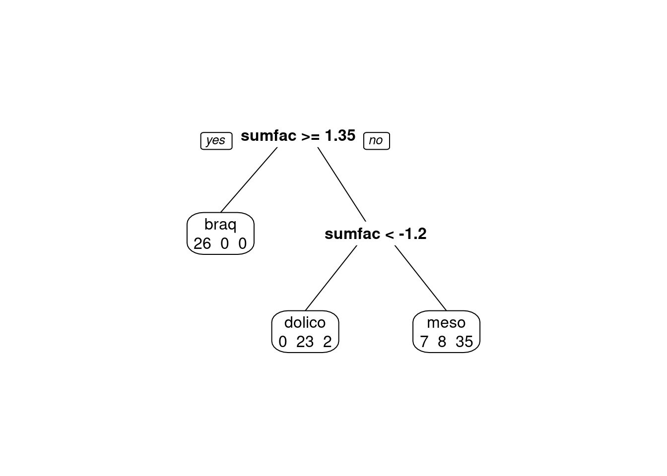
predito = predict(modArvDec01, type = "class")
cm = confusionMatrix(predito, tipofacial$grupo)
cm
## Confusion Matrix and Statistics
##
## Reference
## Prediction braq dolico meso
## braq 26 0 0
## dolico 0 23 2
## meso 7 8 35
##
## Overall Statistics
##
## Accuracy : 0.8317
## 95% CI : (0.7442, 0.8988)
## No Information Rate : 0.3663
## P-Value [Acc > NIR] : < 2.2e-16
##
## Kappa : 0.7444
##
## Mcnemar's Test P-Value : NA
##
## Statistics by Class:
##
## Class: braq Class: dolico Class: meso
## Sensitivity 0.7879 0.7419 0.9459
## Specificity 1.0000 0.9714 0.7656
## Pos Pred Value 1.0000 0.9200 0.7000
## Neg Pred Value 0.9067 0.8947 0.9608
## Prevalence 0.3267 0.3069 0.3663
## Detection Rate 0.2574 0.2277 0.3465
## Detection Prevalence 0.2574 0.2475 0.4950
## Balanced Accuracy 0.8939 0.8567 0.8558# Adiciona as métricas no df
model_eval[nrow(model_eval) + 1,] <- c("modArvDec01", "rpart", cm$overall['Accuracy'], cm$byClass[,1], cm$byClass[,2])x = 1:nrow(tipofacial)
plot(tipofacial$sumfac ~ x, col = tipofacial$grupo)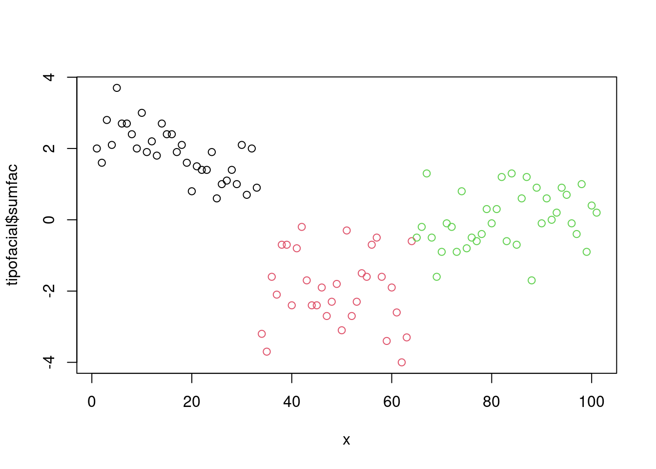
2.5.5.12 SVM
modSVM01 = svm(grupo ~ sumfac, data = tipofacial, kernel = "linear")
predito = predict(modSVM01, type = "class")
cm = confusionMatrix(predito, tipofacial$grupo)

# Adiciona as métricas no df
model_eval[nrow(model_eval) + 1,] <- c("modSVM01", "svm", cm$overall['Accuracy'], cm$byClass[,1], cm$byClass[,2])
2.5.6 rede neural
modRedNeural01 = neuralnet(grupo ~ sumfac, data = tipofacial, hidden = c(2,4,3))
plot(modRedNeural01)

ypred = neuralnet::compute(modRedNeural01, tipofacial)
yhat = ypred$net.result

yhat = round(yhat)

yhat=data.frame("yhat"= dplyr::case_when(yhat[ ,1:1]==1 ~ "braq",
                                         yhat[ ,2:2]==1 ~ "dolico",
                                         TRUE ~ "meso"))

cm = confusionMatrix(tipofacial$grupo, as.factor(yhat$yhat))
cm
## Confusion Matrix and Statistics
##
## Reference
## Prediction braq dolico meso
## braq 30 0 3
## dolico 0 23 8
## meso 3 2 32
##
## Overall Statistics
##
## Accuracy : 0.8416
## 95% CI : (0.7555, 0.9067)
## No Information Rate : 0.4257
## P-Value [Acc > NIR] : < 2.2e-16
##
## Kappa : 0.7605
##
## Mcnemar's Test P-Value : NA
##
## Statistics by Class:
##
## Class: braq Class: dolico Class: meso
## Sensitivity 0.9091 0.9200 0.7442
## Specificity 0.9559 0.8947 0.9138
## Pos Pred Value 0.9091 0.7419 0.8649
## Neg Pred Value 0.9559 0.9714 0.8281
## Prevalence 0.3267 0.2475 0.4257
## Detection Rate 0.2970 0.2277 0.3168
## Detection Prevalence 0.3267 0.3069 0.3663
## Balanced Accuracy 0.9325 0.9074 0.8290# Adiciona as métricas no df
model_eval[nrow(model_eval) + 1,] <- c("modRedNeural01", "neuralnet", cm$overall['Accuracy'], cm$byClass[,1], cm$byClass[,2])2.5.7 KNN
modKnn1_01 = knn3(grupo ~ sumfac, data = tipofacial, k = 1)
predito = predict(modKnn1_01, tipofacial, type = "class")
cm = confusionMatrix(predito, tipofacial$grupo)
cm
## Confusion Matrix and Statistics
##
## Reference
## Prediction braq dolico meso
## braq 33 0 1
## dolico 0 29 4
## meso 0 2 32
##
## Overall Statistics
##
## Accuracy : 0.9307
## 95% CI : (0.8624, 0.9717)
## No Information Rate : 0.3663
## P-Value [Acc > NIR] : < 2.2e-16
##
## Kappa : 0.896
##
## Mcnemar's Test P-Value : NA
##
## Statistics by Class:
##
## Class: braq Class: dolico Class: meso
## Sensitivity 1.0000 0.9355 0.8649
## Specificity 0.9853 0.9429 0.9688
## Pos Pred Value 0.9706 0.8788 0.9412
## Neg Pred Value 1.0000 0.9706 0.9254
## Prevalence 0.3267 0.3069 0.3663
## Detection Rate 0.3267 0.2871 0.3168
## Detection Prevalence 0.3366 0.3267 0.3366
## Balanced Accuracy 0.9926 0.9392 0.9168# Adiciona as métricas no df
model_eval[nrow(model_eval) + 1,] <- c("modKnn1_01-k=1", "knn3", cm$overall['Accuracy'], cm$byClass[,1], cm$byClass[,2])k = 3
modKnn3_01 = knn3(grupo ~ sumfac, data = tipofacial, k = 3)
predito = predict(modKnn3_01, tipofacial, type = "class")
cm = confusionMatrix(predito, tipofacial$grupo, positive = "0")

# Adiciona as métricas no df
model_eval[nrow(model_eval) + 1,] <- c("modKnn3_01-k=3", "knn3", cm$overall['Accuracy'], cm$byClass[,1], cm$byClass[,2])
k = 5
modKnn5_01 = knn3(grupo ~ sumfac, data = tipofacial, k = 5)
predito = predict(modKnn5_01, tipofacial, type = "class")
cm = confusionMatrix(predito, tipofacial$grupo, positive = "0")
cm
## Confusion Matrix and Statistics
##
## Reference
## Prediction braq dolico meso
## braq 30 0 1
## dolico 0 27 4
## meso 3 4 32
##
## Overall Statistics
##
## Accuracy : 0.8812
## 95% CI : (0.8017, 0.9371)
## No Information Rate : 0.3663
## P-Value [Acc > NIR] : < 2.2e-16
##
## Kappa : 0.8211
##
## Mcnemar's Test P-Value : NA
##
## Statistics by Class:
##
## Class: braq Class: dolico Class: meso
## Sensitivity 0.9091 0.8710 0.8649
## Specificity 0.9853 0.9429 0.8906
## Pos Pred Value 0.9677 0.8710 0.8205
## Neg Pred Value 0.9571 0.9429 0.9194
## Prevalence 0.3267 0.3069 0.3663
## Detection Rate 0.2970 0.2673 0.3168
## Detection Prevalence 0.3069 0.3069 0.3861
## Balanced Accuracy 0.9472 0.9069 0.8777# Adiciona as métricas no df
model_eval[nrow(model_eval) + 1,] <- c("modKnn3_01-k=5", "knn3", cm$overall['Accuracy'], cm$byClass[,1], cm$byClass[,2])2.5.8 Avaliando os modelos
| Model | Algorithm | Accuracy | Sensitivity_C1 | Sensitivity_C2 | Sensitivity_C3 | Specificity_C1 | Specificity_C2 | Specificity_C3 |
|---|---|---|---|---|---|---|---|---|
| glm.fit | glm | 0.801980198019802 | 0.818181818181818 | 0.741935483870968 | 0.837837837837838 | 0.941176470588235 | 0.971428571428571 | 0.78125 |
| glm.fit-split | glm | 0.741935483870968 | 0.875 | 0.714285714285714 | 0.6875 | 0.826086956521739 | 0.958333333333333 | 0.8 |
| modFisher01 | lda | 0.811881188118812 | 0.878787878787879 | 0.741935483870968 | 0.810810810810811 | 0.926470588235294 | 0.971428571428571 | 0.8125 |
| modBayes01-prior 0.25 / 0.50 / 0.25 | lda | 0.782178217821782 | 0.878787878787879 | 0.774193548387097 | 0.702702702702703 | 0.926470588235294 | 0.914285714285714 | 0.828125 |
| modNaiveBayes01 | naiveBayes | 0.811881188118812 | 0.878787878787879 | 0.741935483870968 | 0.810810810810811 | 0.926470588235294 | 0.971428571428571 | 0.8125 |
| modArvDec01 | rpart | 0.831683168316832 | 0.787878787878788 | 0.741935483870968 | 0.945945945945946 | 1 | 0.971428571428571 | 0.765625 |
| modSVM01 | svm | 0.801980198019802 | 0.818181818181818 | 0.741935483870968 | 0.837837837837838 | 0.941176470588235 | 0.971428571428571 | 0.78125 |
| modRedNeural01 | neuralnet | 0.841584158415842 | 0.909090909090909 | 0.92 | 0.744186046511628 | 0.955882352941177 | 0.894736842105263 | 0.913793103448276 |
| modKnn1_01-k=1 | knn3 | 0.930693069306931 | 1 | 0.935483870967742 | 0.864864864864865 | 0.985294117647059 | 0.942857142857143 | 0.96875 |
| modKnn3_01-k=3 | knn3 | 0.871287128712871 | 0.939393939393939 | 0.838709677419355 | 0.837837837837838 | 0.955882352941177 | 0.957142857142857 | 0.890625 |
| modKnn3_01-k=5 | knn3 | 0.881188118811881 | 0.909090909090909 | 0.870967741935484 | 0.864864864864865 | 0.985294117647059 | 0.942857142857143 | 0.890625 |
Todos os modelos tiveram uma performace boa considerando knn, com \(k=3\), o resultado foi melhor.
2.5.9 Agrupamento
tipofacialS = subset(tipofacial, select=c("sexo", "idade", "altfac", "proffac"))

dummy <- dummyVars(" ~ .", data=tipofacialS)
newdata <- data.frame(predict(dummy, newdata = tipofacialS))

d <- dist(newdata, method = "maximum")
grup = hclust(d, method = "ward.D")
plot(grup, cex = 0.6)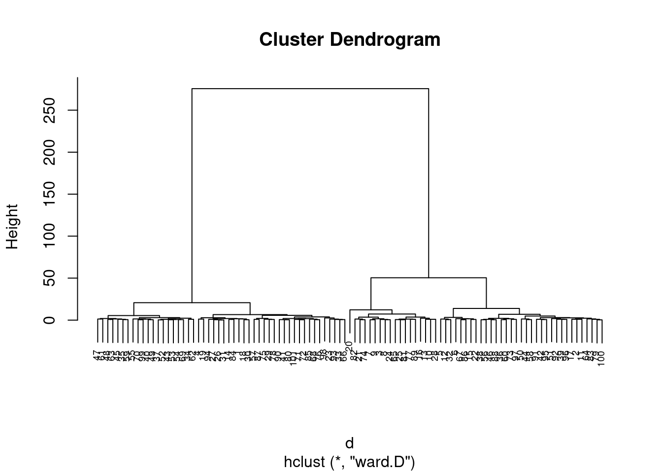
groups <- cutree(grup, k=3)
table(groups, tipofacial$grupo)
##
## groups braq dolico meso
## 1 12 19 19
## 2 9 12 12
## 3 12 0 6km1 = kmeans(newdata, 4)
p1 = fviz_cluster(km1, data=newdata,
palette = c("#2E9FDF", "#FC4E07", "#E7B800", "#E7B700"),
star.plot=FALSE,
# repel=TRUE,
ggtheme=theme_bw())
p1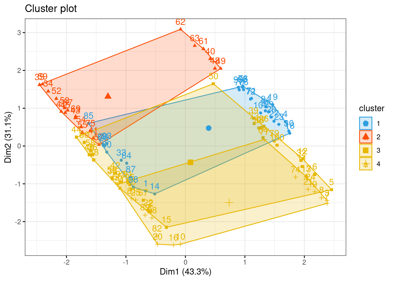
groups = km1$cluster
table(groups, tipofacial$grupo)
##
## groups braq dolico meso
## 1 12 0 17
## 2 0 19 2
## 3 9 12 12
## 4 12 0 62.5.10 Pacotes
Pacotes necessários para estes exercícios:
library(readxl)
library(tidyverse)
library(readxl)
library(ggthemes)
library(plotly)
library(knitr)
library(kableExtra)
library(factoextra)
2.5.10.1 Conjunto de dados
USArrests é um conjunto de dados contendo estatísticas de prisões por 100.000 habitantes por agressão, assassinato e estupro em cada um dos 50 estados dos EUA em 1973. Também é fornecida a porcentagem da população que vive em áreas urbanas.
summary(USArrests)

require(graphics)
pairs(USArrests, panel = panel.smooth, main = "USArrests data")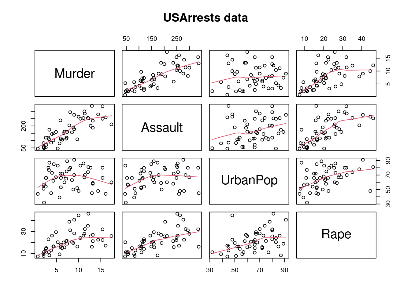
## Difference between 'USArrests' and its correction
USArrests["Maryland", "UrbanPop"] # 67 -- the transcription error
UA.C <- USArrests
UA.C["Maryland", "UrbanPop"] <- 76.6

## also +/- 0.5 to restore the original  <n>.5  percentages
s5u <- c("Colorado", "Florida", "Mississippi", "Wyoming")
s5d <- c("Nebraska", "Pennsylvania")
UA.C[s5u, "UrbanPop"] <- UA.C[s5u, "UrbanPop"] + 0.5
UA.C[s5d, "UrbanPop"] <- UA.C[s5d, "UrbanPop"] - 0.5
2.5.11 Agrupamento
df <- scale(USArrests)

summary(df)
## Murder Assault UrbanPop Rape
## Min. :-1.6044 Min. :-1.5090 Min. :-2.31714 Min. :-1.4874
## 1st Qu.:-0.8525 1st Qu.:-0.7411 1st Qu.:-0.76271 1st Qu.:-0.6574
## Median :-0.1235 Median :-0.1411 Median : 0.03178 Median :-0.1209
## Mean : 0.0000 Mean : 0.0000 Mean : 0.00000 Mean : 0.0000
## 3rd Qu.: 0.7949 3rd Qu.: 0.9388 3rd Qu.: 0.84354 3rd Qu.: 0.5277
## Max. : 2.2069 Max. : 1.9948 Max. : 1.75892 Max. : 2.6444d <- dist(df, method = "maximum")
grup = hclust(d, method = "ward.D")
plot(grup, cex = 0.6)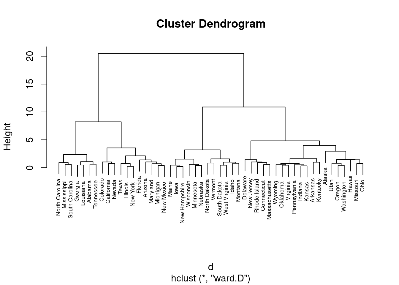
groups <- cutree(grup, k=3)
groups
## Alabama Alaska Arizona Arkansas California Colorado Connecticut
## 1 2 1 2 1 1 2
## Delaware Florida Georgia Hawaii Idaho Illinois Indiana
## 2 1 1 2 3 1 2
## Iowa Kansas Kentucky Louisiana Maine Maryland Massachusetts
## 3 2 2 1 3 1 2
## Michigan Minnesota Mississippi Missouri Montana Nebraska Nevada
## 1 3 1 2 3 3 1
## New Hampshire New Jersey New Mexico New York North Carolina North Dakota Ohio
## 3 2 1 1 1 3 2
## Oklahoma Oregon Pennsylvania Rhode Island South Carolina South Dakota Tennessee
## 2 2 2 2 1 3 1
## Texas Utah Vermont Virginia Washington West Virginia Wisconsin
## 1 2 3 2 2 3 3
## Wyoming
## 2km1 = kmeans(df, 4, nstart = 25)
km1## K-means clustering with 4 clusters of sizes 13, 16, 8, 13
##
## Cluster means:
## Murder Assault UrbanPop Rape
## 1 -0.9615407 -1.1066010 -0.9301069 -0.96676331
## 2 -0.4894375 -0.3826001 0.5758298 -0.26165379
## 3 1.4118898 0.8743346 -0.8145211 0.01927104
## 4 0.6950701 1.0394414 0.7226370 1.27693964
##
## Clustering vector:
## Alabama Alaska Arizona Arkansas California Colorado Connecticut
## 3 4 4 3 4 4 2
## Delaware Florida Georgia Hawaii Idaho Illinois Indiana
## 2 4 3 2 1 4 2
## Iowa Kansas Kentucky Louisiana Maine Maryland Massachusetts
## 1 2 1 3 1 4 2
## Michigan Minnesota Mississippi Missouri Montana Nebraska Nevada
## 4 1 3 4 1 1 4
## New Hampshire New Jersey New Mexico New York North Carolina North Dakota Ohio
## 1 2 4 4 3 1 2
## Oklahoma Oregon Pennsylvania Rhode Island South Carolina South Dakota Tennessee
## 2 2 2 2 3 1 3
## Texas Utah Vermont Virginia Washington West Virginia Wisconsin
## 4 2 1 2 2 1 1
## Wyoming
## 2
##
## Within cluster sum of squares by cluster:
## [1] 11.952463 16.212213 8.316061 19.922437
## (between_SS / total_SS = 71.2 %)
##
## Available components:
##
## [1] "cluster" "centers" "totss" "withinss" "tot.withinss" "betweenss" "size"
## [8] "iter" "ifault"aggregate(df, by=list(cluster=km1$cluster), mean)## cluster Murder Assault UrbanPop Rape
## 1 1 -0.9615407 -1.1066010 -0.9301069 -0.96676331
## 2 2 -0.4894375 -0.3826001 0.5758298 -0.26165379
## 3 3 1.4118898 0.8743346 -0.8145211 0.01927104
## 4 4 0.6950701 1.0394414 0.7226370 1.27693964p1 = fviz_cluster(km1, data=df,
palette = c("#2E9FDF", "#FC4E07", "#E7B800", "#E7B700"),
star.plot=FALSE,
# repel=TRUE,
ggtheme=theme_bw(),
main = "Particionamento")
p1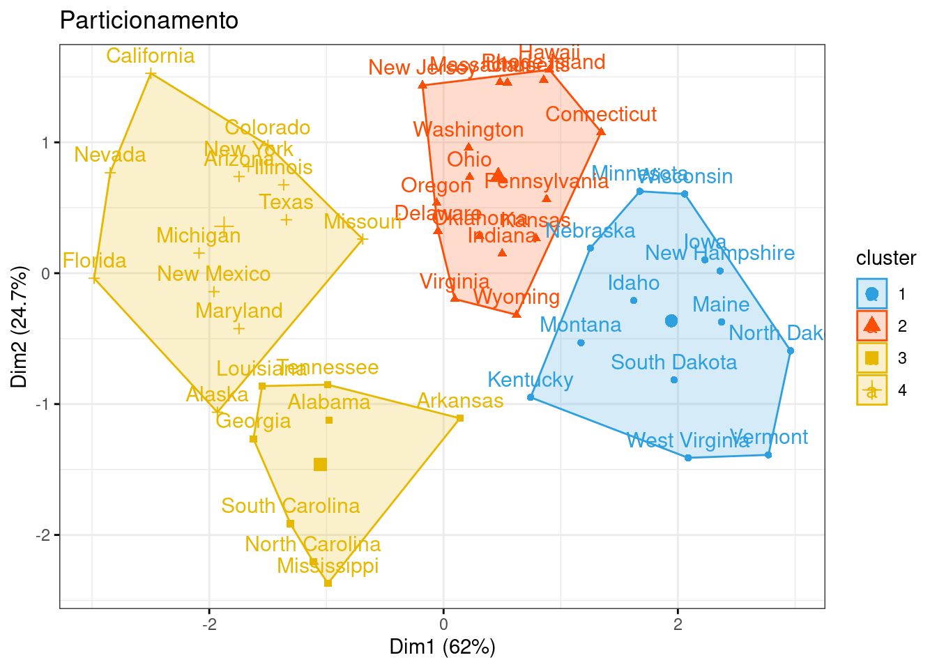
2.5.12 Conjunto de dados
#GET("http://www.ime.usp.br/~jmsinger/MorettinSinger/inibina.xls", write_disk(tf <- tempfile(fileext = ".xls")))
httr::GET("http://www.ime.usp.br/~jmsinger/MorettinSinger/inibina.xls", httr::write_disk("Dados/inibina.xls", overwrite = TRUE))
## Response [https://www.ime.usp.br/~jmsinger/MorettinSinger/inibina.xls]
## Date: 2022-12-13 23:42
## Status: 200
## Content-Type: application/vnd.ms-excel
## Size: 8.7 kB
## <ON DISK> /home/emau/R/Caderno_Eder/BIG019_Eder/Dados/inibina.xlsinibina <- read_excel("Dados/inibina.xls")
str(inibina)## tibble [32 × 4] (S3: tbl_df/tbl/data.frame)
## $ ident : num [1:32] 1 2 3 4 5 6 7 8 9 10 ...
## $ resposta: chr [1:32] "positiva" "positiva" "positiva" "positiva" ...
## $ inibpre : num [1:32] 54 159.1 98.3 85.3 127.9 ...
## $ inibpos : num [1:32] 65.9 281.1 305.4 434.4 229.3 ...nrow(inibina)## [1] 32sum()## [1] 0inibina$difinib = inibina$inibpos - inibina$inibpre
inibina$resposta = as.factor(inibina$resposta)plot(inibina$difinib ~ inibina$resposta, ylim = c(0, 400))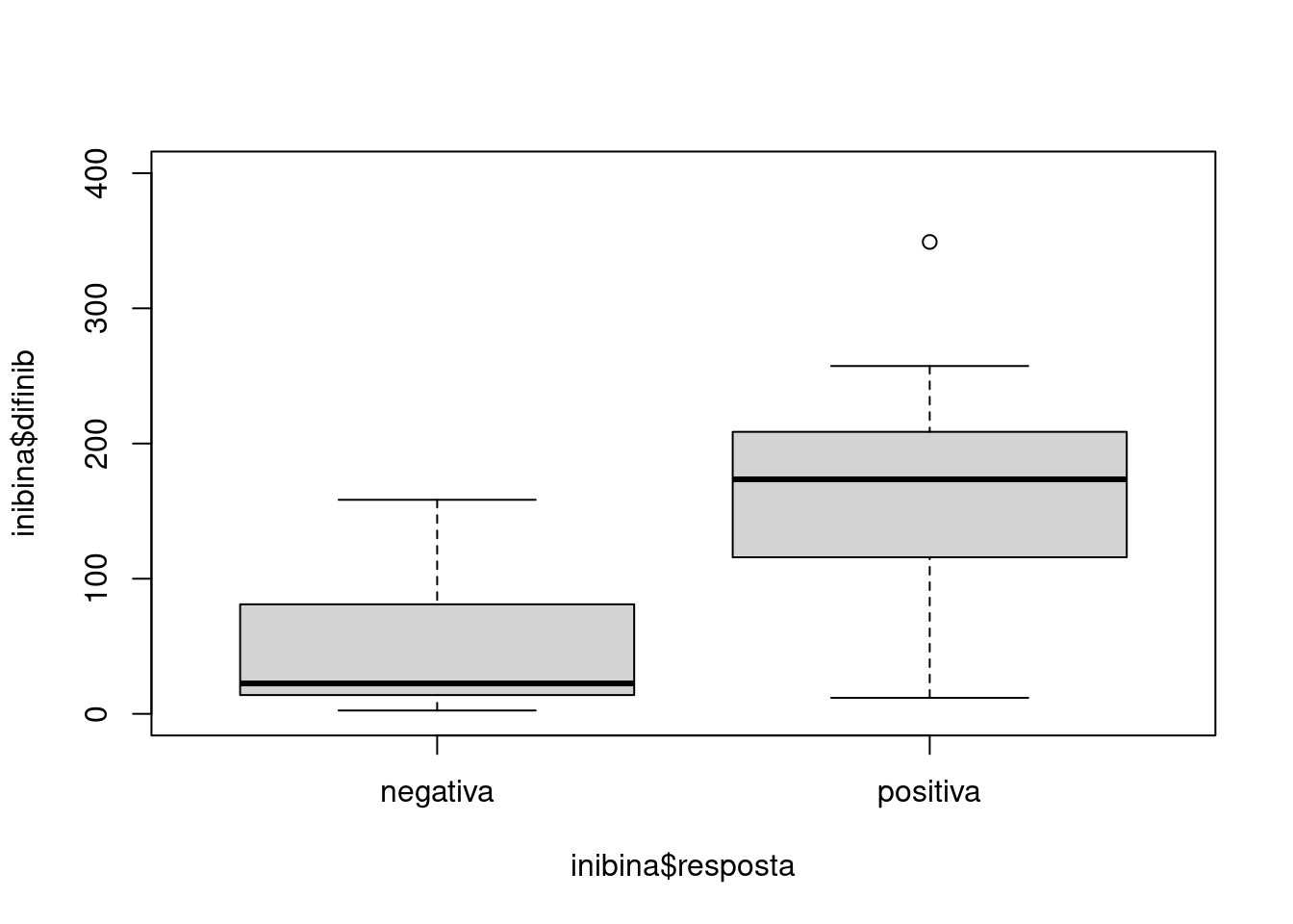
print(inibina, n = 32)## # A tibble: 32 × 5
## ident resposta inibpre inibpos difinib
## <dbl> <fct> <dbl> <dbl> <dbl>
## 1 1 positiva 54.0 65.9 11.9
## 2 2 positiva 159. 281. 122.
## 3 3 positiva 98.3 305. 207.
## 4 4 positiva 85.3 434. 349.
## 5 5 positiva 128. 229. 101.
## 6 6 positiva 144. 354. 210.
## 7 7 positiva 111. 254. 143.
## 8 8 positiva 47.5 199. 152.
## 9 9 positiva 123. 328. 205.
## 10 10 positiva 166. 339. 174.
## 11 11 positiva 145. 377. 232.
## 12 12 positiva 186. 1055. 869.
## 13 13 positiva 149. 354. 204.
## 14 14 positiva 33.3 100. 66.8
## 15 15 positiva 182. 358. 177.
## 16 16 positiva 58.4 168. 110.
## 17 17 positiva 128. 228. 100.
## 18 18 positiva 153. 312. 159.
## 19 19 positiva 149. 406. 257.
## 20 20 negativa 81 201. 120.
## 21 21 negativa 24.7 45.2 20.4
## 22 22 negativa 3.02 6.03 3.01
## 23 23 negativa 4.27 17.8 13.5
## 24 24 negativa 99.3 128. 28.6
## 25 25 negativa 108. 129. 21.1
## 26 26 negativa 7.36 21.3 13.9
## 27 27 negativa 161. 320. 158.
## 28 28 negativa 184. 311. 127.
## 29 29 negativa 23.1 45.6 22.5
## 30 30 negativa 111. 192. 81.0
## 31 31 negativa 106. 131. 24.8
## 32 32 negativa 3.98 6.46 2.48# Hmisc::describe(inibina)
summary(inibina)## ident resposta inibpre inibpos difinib
## Min. : 1.00 negativa:13 Min. : 3.02 Min. : 6.03 Min. : 2.48
## 1st Qu.: 8.75 positiva:19 1st Qu.: 52.40 1st Qu.: 120.97 1st Qu.: 24.22
## Median :16.50 Median :109.44 Median : 228.89 Median :121.18
## Mean :16.50 Mean :100.53 Mean : 240.80 Mean :140.27
## 3rd Qu.:24.25 3rd Qu.:148.93 3rd Qu.: 330.77 3rd Qu.:183.77
## Max. :32.00 Max. :186.38 Max. :1055.19 Max. :868.81sd(inibina$difinib)## [1] 159.2217Gerando dataframe para comparar as métricas entre os modelos.
model_eval <- data.frame(matrix(ncol = 5, nrow = 0))

colnames(model_eval) <- c('Model', 'Algorithm', 'Accuracy', 'Sensitivity', 'Specificity')
2.5.13 Generalizando Modelos Lineares
modLogist01 = glm(resposta ~ difinib, family = binomial, data = inibina)
summary(modLogist01)
##
## Call:
## glm(formula = resposta ~ difinib, family = binomial, data = inibina)
##
## Deviance Residuals:
## Min 1Q Median 3Q Max
## -1.9770 -0.5594 0.1890 0.5589 2.0631
##
## Coefficients:
## Estimate Std. Error z value Pr(>|z|)
## (Intercept) -2.310455 0.947438 -2.439 0.01474 *
## difinib 0.025965 0.008561 3.033 0.00242 **
## ---
## Signif. codes: 0 '***' 0.001 '**' 0.01 '*' 0.05 '.' 0.1 ' ' 1
##
## (Dispersion parameter for binomial family taken to be 1)
##
## Null deviance: 43.230 on 31 degrees of freedom
## Residual deviance: 24.758 on 30 degrees of freedom
## AIC: 28.758
##
## Number of Fisher Scoring iterations: 6predito = predict.glm(modLogist01, type = "response")
classPred = ifelse(predito>0.5, "positiva", "negativa")
classPred = as.factor(classPred)
cm = confusionMatrix(classPred, inibina$resposta, positive = "positiva")
cm## Confusion Matrix and Statistics
##
## Reference
## Prediction negativa positiva
## negativa 10 2
## positiva 3 17
##
## Accuracy : 0.8438
## 95% CI : (0.6721, 0.9472)
## No Information Rate : 0.5938
## P-Value [Acc > NIR] : 0.002273
##
## Kappa : 0.6721
##
## Mcnemar's Test P-Value : 1.000000
##
## Sensitivity : 0.8947
## Specificity : 0.7692
## Pos Pred Value : 0.8500
## Neg Pred Value : 0.8333
## Prevalence : 0.5938
## Detection Rate : 0.5312
## Detection Prevalence : 0.6250
## Balanced Accuracy : 0.8320
##
## 'Positive' Class : positiva
## # Adiciona as métricas no df
model_eval[nrow(model_eval) + 1,] <- c("modLogist01", "glm", cm$overall['Accuracy'], cm$byClass['Sensitivity'], cm$byClass['Specificity'])Validação cruzada leave-one-out
trControl <- trainControl(method = "LOOCV")

modLogist02 <- train(resposta ~ difinib, method = "glm", data = inibina, family = binomial,
                     trControl = trControl, metric = "Accuracy")
summary(modLogist02)
##
## Call:
## NULL
##
## Deviance Residuals:
## Min 1Q Median 3Q Max
## -1.9770 -0.5594 0.1890 0.5589 2.0631
##
## Coefficients:
## Estimate Std. Error z value Pr(>|z|)
## (Intercept) -2.310455 0.947438 -2.439 0.01474 *
## difinib 0.025965 0.008561 3.033 0.00242 **
## ---
## Signif. codes: 0 '***' 0.001 '**' 0.01 '*' 0.05 '.' 0.1 ' ' 1
##
## (Dispersion parameter for binomial family taken to be 1)
##
## Null deviance: 43.230 on 31 degrees of freedom
## Residual deviance: 24.758 on 30 degrees of freedom
## AIC: 28.758
##
## Number of Fisher Scoring iterations: 6predito = predict(modLogist02, newdata = inibina)
classPred = as.factor(predito)
cm = confusionMatrix(classPred, inibina$resposta, positive = "positiva")
cm## Confusion Matrix and Statistics
##
## Reference
## Prediction negativa positiva
## negativa 10 2
## positiva 3 17
##
## Accuracy : 0.8438
## 95% CI : (0.6721, 0.9472)
## No Information Rate : 0.5938
## P-Value [Acc > NIR] : 0.002273
##
## Kappa : 0.6721
##
## Mcnemar's Test P-Value : 1.000000
##
## Sensitivity : 0.8947
## Specificity : 0.7692
## Pos Pred Value : 0.8500
## Neg Pred Value : 0.8333
## Prevalence : 0.5938
## Detection Rate : 0.5312
## Detection Prevalence : 0.6250
## Balanced Accuracy : 0.8320
##
## 'Positive' Class : positiva
## # Adiciona as métricas no df
model_eval[nrow(model_eval) + 1,] <- c("modLogist02-LOOCV", "glm", cm$overall['Accuracy'], cm$byClass['Sensitivity'], cm$byClass['Specificity'])Treinar o modelo com o método LOOCV como demonstrado em aula porem não mudou o resultado.
2.5.14 Analise Descri. Linear - Fisher
modFisher01 = lda(resposta ~ difinib, data = inibina, prior = c(0.5, 0.5))
predito = predict(modFisher01)
classPred = predito$class
cm = confusionMatrix(classPred, inibina$resposta, positive = "positiva")
cm
## Confusion Matrix and Statistics
##
## Reference
## Prediction negativa positiva
## negativa 11 6
## positiva 2 13
##
## Accuracy : 0.75
## 95% CI : (0.566, 0.8854)
## No Information Rate : 0.5938
## P-Value [Acc > NIR] : 0.04978
##
## Kappa : 0.5058
##
## Mcnemar's Test P-Value : 0.28884
##
## Sensitivity : 0.6842
## Specificity : 0.8462
## Pos Pred Value : 0.8667
## Neg Pred Value : 0.6471
## Prevalence : 0.5938
## Detection Rate : 0.4062
## Detection Prevalence : 0.4688
## Balanced Accuracy : 0.7652
##
## 'Positive' Class : positiva
## # Adiciona as métricas no df
model_eval[nrow(model_eval) + 1,] <- c("modFisher01-prior 0.5 / 0.5", "lda", cm$overall['Accuracy'], cm$byClass['Sensitivity'], cm$byClass['Specificity'])2.5.15 Bayes
inibina$resposta## [1] positiva positiva positiva positiva positiva positiva positiva positiva positiva positiva positiva positiva
## [13] positiva positiva positiva positiva positiva positiva positiva negativa negativa negativa negativa negativa
## [25] negativa negativa negativa negativa negativa negativa negativa negativa
## Levels: negativa positivamodBayes01 = lda(resposta ~ difinib, data = inibina, prior = c(0.65, 0.35))
predito = predict(modBayes01)
classPred = predito$class
cm = confusionMatrix(classPred, inibina$resposta, positive = "positiva")
cm## Confusion Matrix and Statistics
##
## Reference
## Prediction negativa positiva
## negativa 13 13
## positiva 0 6
##
## Accuracy : 0.5938
## 95% CI : (0.4064, 0.763)
## No Information Rate : 0.5938
## P-Value [Acc > NIR] : 0.5755484
##
## Kappa : 0.2727
##
## Mcnemar's Test P-Value : 0.0008741
##
## Sensitivity : 0.3158
## Specificity : 1.0000
## Pos Pred Value : 1.0000
## Neg Pred Value : 0.5000
## Prevalence : 0.5938
## Detection Rate : 0.1875
## Detection Prevalence : 0.1875
## Balanced Accuracy : 0.6579
##
## 'Positive' Class : positiva
## # Adiciona as métricas no df
model_eval[nrow(model_eval) + 1,] <- c("modBayes01-prior 0.65 / 0.35", "lda", cm$overall['Accuracy'], cm$byClass['Sensitivity'], cm$byClass['Specificity'])table(classPred)## classPred
## negativa positiva
## 26 6print(inibina, n = 32)## # A tibble: 32 × 5
## ident resposta inibpre inibpos difinib
## <dbl> <fct> <dbl> <dbl> <dbl>
## 1 1 positiva 54.0 65.9 11.9
## 2 2 positiva 159. 281. 122.
## 3 3 positiva 98.3 305. 207.
## 4 4 positiva 85.3 434. 349.
## 5 5 positiva 128. 229. 101.
## 6 6 positiva 144. 354. 210.
## 7 7 positiva 111. 254. 143.
## 8 8 positiva 47.5 199. 152.
## 9 9 positiva 123. 328. 205.
## 10 10 positiva 166. 339. 174.
## 11 11 positiva 145. 377. 232.
## 12 12 positiva 186. 1055. 869.
## 13 13 positiva 149. 354. 204.
## 14 14 positiva 33.3 100. 66.8
## 15 15 positiva 182. 358. 177.
## 16 16 positiva 58.4 168. 110.
## 17 17 positiva 128. 228. 100.
## 18 18 positiva 153. 312. 159.
## 19 19 positiva 149. 406. 257.
## 20 20 negativa 81 201. 120.
## 21 21 negativa 24.7 45.2 20.4
## 22 22 negativa 3.02 6.03 3.01
## 23 23 negativa 4.27 17.8 13.5
## 24 24 negativa 99.3 128. 28.6
## 25 25 negativa 108. 129. 21.1
## 26 26 negativa 7.36 21.3 13.9
## 27 27 negativa 161. 320. 158.
## 28 28 negativa 184. 311. 127.
## 29 29 negativa 23.1 45.6 22.5
## 30 30 negativa 111. 192. 81.0
## 31 31 negativa 106. 131. 24.8
## 32 32 negativa 3.98 6.46 2.48Naive Bayes
modNaiveBayes01 = naiveBayes(resposta ~ difinib, data = inibina)
predito = predict(modNaiveBayes01, inibina)
cm = confusionMatrix(predito, inibina$resposta, positive = "positiva")
cm
## Confusion Matrix and Statistics
##
## Reference
## Prediction negativa positiva
## negativa 11 5
## positiva 2 14
##
## Accuracy : 0.7812
## 95% CI : (0.6003, 0.9072)
## No Information Rate : 0.5938
## P-Value [Acc > NIR] : 0.02102
##
## Kappa : 0.5625
##
## Mcnemar's Test P-Value : 0.44969
##
## Sensitivity : 0.7368
## Specificity : 0.8462
## Pos Pred Value : 0.8750
## Neg Pred Value : 0.6875
## Prevalence : 0.5938
## Detection Rate : 0.4375
## Detection Prevalence : 0.5000
## Balanced Accuracy : 0.7915
##
## 'Positive' Class : positiva
## # Adiciona as métricas no df
model_eval[nrow(model_eval) + 1,] <- c("modNaiveBayes01", "naiveBayes", cm$overall['Accuracy'], cm$byClass['Sensitivity'], cm$byClass['Specificity'])2.5.16 Arvore de Decisao
modArvDec01 = rpart(resposta ~ difinib, data = inibina)
prp(modArvDec01,  faclen=0, #use full names for factor labels
    extra=1, #display number of observations for each terminal node
    roundint=F, #don't round to integers in output
    digits=5)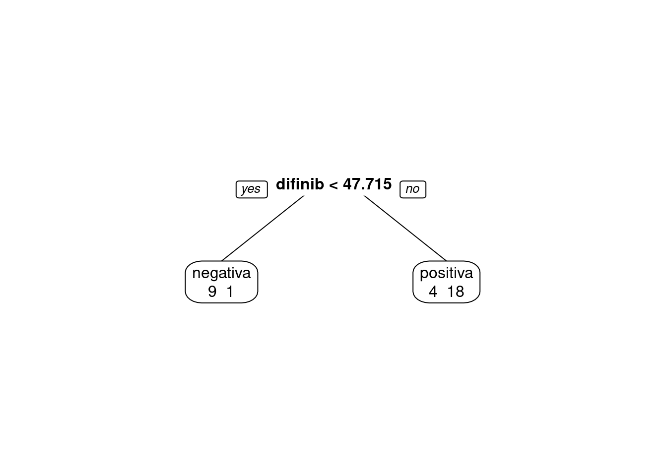
predito = predict(modArvDec01, type = "class")
cm = confusionMatrix(predito, inibina$resposta, positive = "positiva")
cm
## Confusion Matrix and Statistics
##
## Reference
## Prediction negativa positiva
## negativa 9 1
## positiva 4 18
##
## Accuracy : 0.8438
## 95% CI : (0.6721, 0.9472)
## No Information Rate : 0.5938
## P-Value [Acc > NIR] : 0.002273
##
## Kappa : 0.6639
##
## Mcnemar's Test P-Value : 0.371093
##
## Sensitivity : 0.9474
## Specificity : 0.6923
## Pos Pred Value : 0.8182
## Neg Pred Value : 0.9000
## Prevalence : 0.5938
## Detection Rate : 0.5625
## Detection Prevalence : 0.6875
## Balanced Accuracy : 0.8198
##
## 'Positive' Class : positiva
## # Adiciona as métricas no df
model_eval[nrow(model_eval) + 1,] <- c("modArvDec01", "rpart", cm$overall['Accuracy'], cm$byClass['Sensitivity'], cm$byClass['Specificity'])x = 1:32
plot(inibina$difinib ~x, col = inibina$resposta)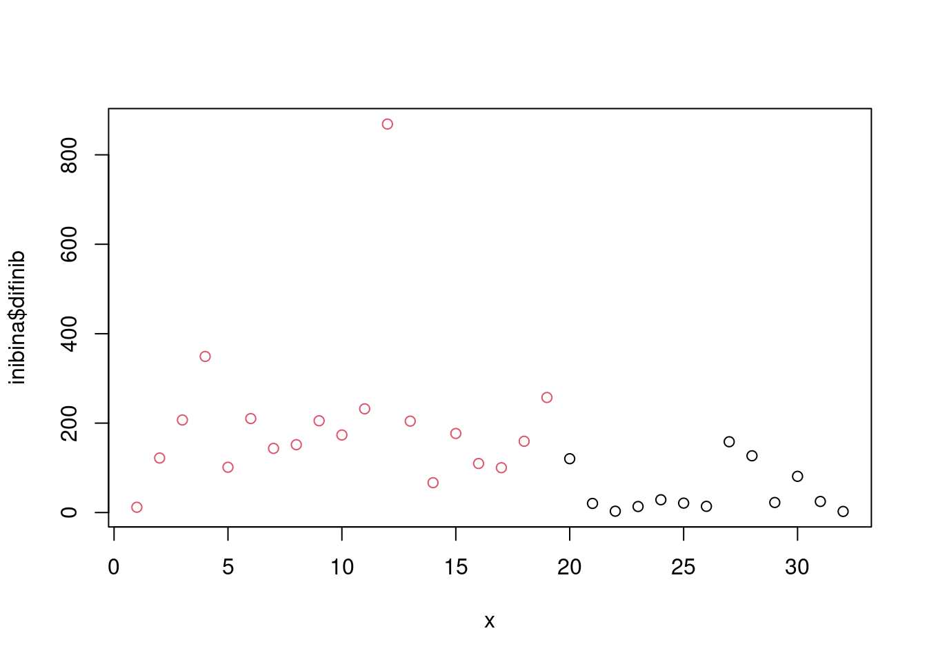
2.5.17 SVM
modSVM01 = svm(resposta ~ difinib, data = inibina, kernel = "linear")
predito = predict(modSVM01, type = "class")
cm = confusionMatrix(predito, inibina$resposta, positive = "positiva")

# Adiciona as métricas no df
model_eval[nrow(model_eval) + 1,] <- c("modSVM01", "svm", cm$overall['Accuracy'], cm$byClass['Sensitivity'], cm$byClass['Specificity'])
2.5.18 neuralnet
modRedNeural01 = neuralnet(resposta ~ difinib, data = inibina, hidden = c(2,4,3))
plot(modRedNeural01)

ypred = neuralnet::compute(modRedNeural01, inibina)
yhat = ypred$net.result

round(yhat)
## [,1] [,2]
## [1,] 0 1
## [2,] 0 1
## [3,] 0 1
## [4,] 0 1
## [5,] 0 1
## [6,] 0 1
## [7,] 0 1
## [8,] 0 1
## [9,] 0 1
## [10,] 0 1
## [11,] 0 1
## [12,] 0 1
## [13,] 0 1
## [14,] 0 1
## [15,] 0 1
## [16,] 0 1
## [17,] 0 1
## [18,] 0 1
## [19,] 0 1
## [20,] 0 1
## [21,] 0 1
## [22,] 0 1
## [23,] 0 1
## [24,] 0 1
## [25,] 0 1
## [26,] 0 1
## [27,] 0 1
## [28,] 0 1
## [29,] 0 1
## [30,] 0 1
## [31,] 0 1
## [32,] 0 1yhat=data.frame("yhat"=ifelse(max.col(yhat[ ,1:2])==1, "negativa", "positiva"))
#cm = confusionMatrix(inibina$resposta, as.factor(yhat$yhat))
cm## Confusion Matrix and Statistics
##
## Reference
## Prediction negativa positiva
## negativa 10 2
## positiva 3 17
##
## Accuracy : 0.8438
## 95% CI : (0.6721, 0.9472)
## No Information Rate : 0.5938
## P-Value [Acc > NIR] : 0.002273
##
## Kappa : 0.6721
##
## Mcnemar's Test P-Value : 1.000000
##
## Sensitivity : 0.8947
## Specificity : 0.7692
## Pos Pred Value : 0.8500
## Neg Pred Value : 0.8333
## Prevalence : 0.5938
## Detection Rate : 0.5312
## Detection Prevalence : 0.6250
## Balanced Accuracy : 0.8320
##
## 'Positive' Class : positiva
## # Adiciona as métricas no df
model_eval[nrow(model_eval) + 1,] <- c("modRedNeural01", "neuralnet", cm$overall['Accuracy'], cm$byClass['Sensitivity'], cm$byClass['Specificity'])2.5.19 KNN
modKnn1_01 = knn3(resposta ~ difinib, data = inibina, k = 1)
predito = predict(modKnn1_01, inibina, type = "class")
cm = confusionMatrix(predito, inibina$resposta, positive = "positiva")
cm
## Confusion Matrix and Statistics
##
## Reference
## Prediction negativa positiva
## negativa 13 0
## positiva 0 19
##
## Accuracy : 1
## 95% CI : (0.8911, 1)
## No Information Rate : 0.5938
## P-Value [Acc > NIR] : 5.693e-08
##
## Kappa : 1
##
## Mcnemar's Test P-Value : NA
##
## Sensitivity : 1.0000
## Specificity : 1.0000
## Pos Pred Value : 1.0000
## Neg Pred Value : 1.0000
## Prevalence : 0.5938
## Detection Rate : 0.5938
## Detection Prevalence : 0.5938
## Balanced Accuracy : 1.0000
##
## 'Positive' Class : positiva
## # Adiciona as métricas no df
model_eval[nrow(model_eval) + 1,] <- c("modKnn1_01-k=1", "knn3", cm$overall['Accuracy'], cm$byClass['Sensitivity'], cm$byClass['Specificity'])k = 3
modKnn3_01 = knn3(resposta ~ difinib, data = inibina, k = 3)
predito = predict(modKnn3_01, inibina, type = "class")
cm = confusionMatrix(predito, inibina$resposta, positive = "positiva")

# Adiciona as métricas no df
model_eval[nrow(model_eval) + 1,] <- c("modKnn3_01-k=3", "knn3", cm$overall['Accuracy'], cm$byClass['Sensitivity'], cm$byClass['Specificity'])
k = 5
modKnn5_01 = knn3(resposta ~ difinib, data = inibina, k = 5)
predito = predict(modKnn5_01, inibina, type = "class")
cm = confusionMatrix(predito, inibina$resposta, positive = "positiva")
cm
## Confusion Matrix and Statistics
##
## Reference
## Prediction negativa positiva
## negativa 9 1
## positiva 4 18
##
## Accuracy : 0.8438
## 95% CI : (0.6721, 0.9472)
## No Information Rate : 0.5938
## P-Value [Acc > NIR] : 0.002273
##
## Kappa : 0.6639
##
## Mcnemar's Test P-Value : 0.371093
##
## Sensitivity : 0.9474
## Specificity : 0.6923
## Pos Pred Value : 0.8182
## Neg Pred Value : 0.9000
## Prevalence : 0.5938
## Detection Rate : 0.5625
## Detection Prevalence : 0.6875
## Balanced Accuracy : 0.8198
##
## 'Positive' Class : positiva
## # Adiciona as métricas no df
model_eval[nrow(model_eval) + 1,] <- c("modKnn5_01-k=5", "knn3", cm$overall['Accuracy'], cm$byClass['Sensitivity'], cm$byClass['Specificity'])2.5.20 Avaliando os modelos
| Model | Algorithm | Accuracy | Sensitivity | Specificity |
|---|---|---|---|---|
| modLogist01 | glm | 0.84375 | 0.894736842105263 | 0.769230769230769 |
| modLogist02-LOOCV | glm | 0.84375 | 0.894736842105263 | 0.769230769230769 |
| modFisher01-prior 0.5 / 0.5 | lda | 0.75 | 0.684210526315789 | 0.846153846153846 |
| modBayes01-prior 0.65 / 0.35 | lda | 0.59375 | 0.315789473684211 | 1 |
| modNaiveBayes01 | naiveBayes | 0.78125 | 0.736842105263158 | 0.846153846153846 |
| modArvDec01 | rpart | 0.84375 | 0.947368421052632 | 0.692307692307692 |
| modSVM01 | svm | 0.84375 | 0.894736842105263 | 0.769230769230769 |
| modRedNeural01 | neuralnet | 0.84375 | 0.894736842105263 | 0.769230769230769 |
| modKnn1_01-k=1 | knn3 | 1 | 1 | 1 |
| modKnn3_01-k=3 | knn3 | 0.875 | 0.894736842105263 | 0.846153846153846 |
| modKnn5_01-k=5 | knn3 | 0.84375 | 0.947368421052632 | 0.692307692307692 |
Os modelos modLogist01, modFisher01 com \(prior = 0.5, 0.5\), modArvDec01 e modKnn3_01 com \(k=3\) resultaram em uma performance simila. Possivlementeo modKnn3_01 apresentou melhor acurácia e especificidade.
2.5.21 Agrupamento
inibinaS = inibina[, 3:5]

d <- dist(inibinaS, method = "maximum")
grup = hclust(d, method = "ward.D")
plot(grup, cex = 0.6)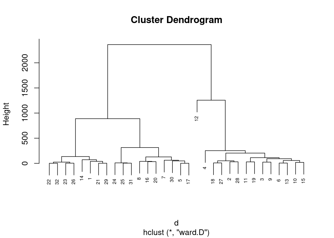
groups <- cutree(grup, k=3)table(groups, inibina$resposta)##
## groups negativa positiva
## 1 11 7
## 2 2 11
## 3 0 1km1 = kmeans(inibinaS, 4)
p1 = fviz_cluster(km1, data=inibinaS,
palette = c("#2E9FDF", "#FC4E07", "#E7B800", "#E7B700"),
star.plot=FALSE,
# repel=TRUE,
ggtheme=theme_bw())
p1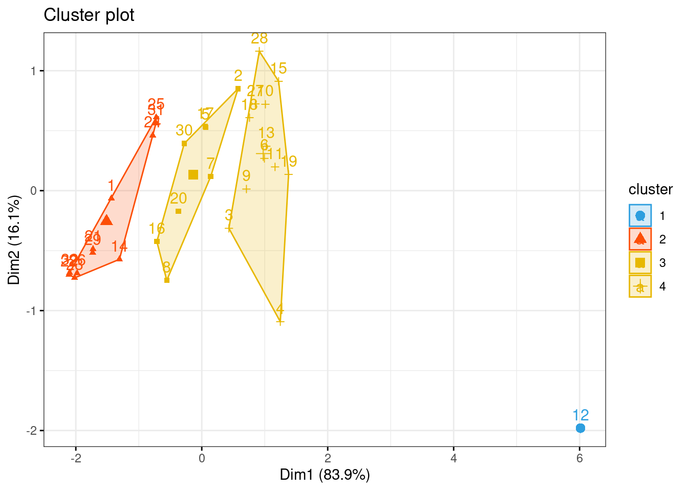
groups = km1$cluster
table(groups, inibina$resposta)
##
## groups negativa positiva
## 1 0 1
## 2 9 2
## 3 2 6
## 4 2 102.5.21.0.0.1 Ultrassom para medir deslocamento do disco
Os dados disponíveis aqui foram extraídos de um estudo realizado no Hospital Universitário da Universidade de São Paulo com o objetivo de avaliar se algumas medidas obtidas ultrassonograficamente poderiam ser utilizadas como substitutas de medidas obtidas por métodos de ressonância magnética, considerada como padrão ouro para avaliação do deslocamento do disco da articulação temporomandibular (referido simplesmente como disco).
2.5.22 Pacotes
Pacotes necessários para estes exercícios:
library(readxl)
library(tidyverse)
library(readxl)
library(ggthemes)
library(plotly)
library(knitr)
library(kableExtra)
library(rpart)
library(rpart.plot)
library(caret)
library(MASS)
library(httr)
library(readxl)
library(tibble)
library(e1071)
library(neuralnet)
library(factoextra)
library(ggpubr)
2.5.22.1 Conjunto de dados
#GET("http://www.ime.usp.br/~jmsinger/MorettinSinger/disco.xls", write_disk(tf <- tempfile(fileext = ".xls")))
httr::GET("http://www.ime.usp.br/~jmsinger/MorettinSinger/disco.xls", httr::write_disk("Dados/disco.xls", overwrite = TRUE))
## Response [https://www.ime.usp.br/~jmsinger/MorettinSinger/disco.xls]
## Date: 2022-12-13 23:42
## Status: 200
## Content-Type: application/vnd.ms-excel
## Size: 11.3 kB
## <ON DISK> /home/emau/R/Caderno_Eder/BIG019_Eder/Dados/disco.xlsdisco <- read_excel("Dados/disco.xls")
str(disco)## tibble [104 × 3] (S3: tbl_df/tbl/data.frame)
## $ deslocamento: num [1:104] 0 0 0 1 0 1 0 0 0 0 ...
## $ distanciaA : num [1:104] 2.2 2.4 2.6 3.5 1.3 2.8 1.5 2.6 1.2 1.7 ...
## $ distanciaF : num [1:104] 1.4 1.2 2 1.8 1 1.1 1.2 1.1 0.6 1.5 ...Número de observações 104.
2.5.22.2 Categorizando a variável de deslocamento.
disco$sumdistancia = disco$distanciaA + disco$distanciaF
disco$deslocamento = as.factor(disco$deslocamento)plot(disco$sumdistancia ~ disco$deslocamento)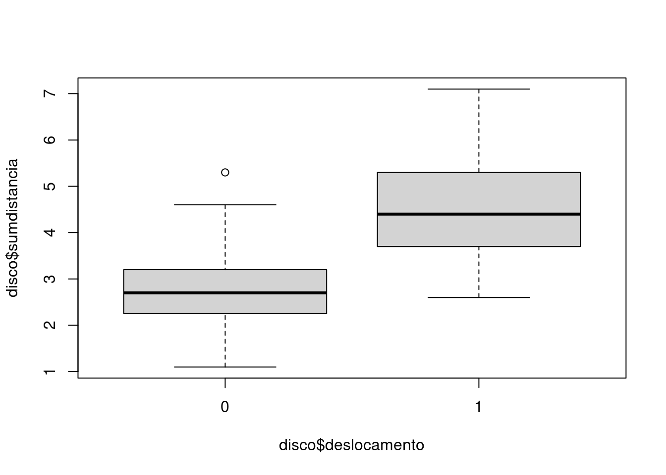
print(disco, n = 32)## # A tibble: 104 × 4
## deslocamento distanciaA distanciaF sumdistancia
## <fct> <dbl> <dbl> <dbl>
## 1 0 2.2 1.4 3.6
## 2 0 2.4 1.2 3.6
## 3 0 2.6 2 4.6
## 4 1 3.5 1.8 5.3
## 5 0 1.3 1 2.3
## 6 1 2.8 1.1 3.9
## 7 0 1.5 1.2 2.7
## 8 0 2.6 1.1 3.7
## 9 0 1.2 0.6 1.8
## 10 0 1.7 1.5 3.2
## 11 0 1.3 1.2 2.5
## 12 0 1.2 1 2.2
## 13 1 4 2.5 6.5
## 14 0 1.2 1 2.2
## 15 1 3.1 1.7 4.8
## 16 1 2.6 0.6 3.2
## 17 0 1.8 0.8 2.6
## 18 0 1.2 1 2.2
## 19 0 1.9 1 2.9
## 20 0 1.2 0.9 2.1
## 21 1 1.7 0.9 2.6
## 22 0 1.2 0.8 2
## 23 1 3.9 3.2 7.1
## 24 0 1.7 1.1 2.8
## 25 0 1.4 1 2.4
## 26 0 1.6 1.3 2.9
## 27 0 1.3 0.5 1.8
## 28 0 1.7 0.7 2.4
## 29 1 2.6 1.8 4.4
## 30 0 1.5 1.5 3
## 31 0 1.8 1.4 3.2
## 32 0 1.2 0.9 2.1
## # … with 72 more rowssummary(disco)## deslocamento distanciaA distanciaF sumdistancia
## 0:75 Min. :0.500 Min. :0.400 Min. :1.100
## 1:29 1st Qu.:1.400 1st Qu.:1.000 1st Qu.:2.500
## Median :1.700 Median :1.200 Median :2.900
## Mean :1.907 Mean :1.362 Mean :3.268
## 3rd Qu.:2.300 3rd Qu.:1.600 3rd Qu.:3.700
## Max. :4.900 Max. :3.300 Max. :7.100sd(disco$sumdistancia)## [1] 1.183976Criando um dataframe para comparar as métricas dos modelos.
model_eval <- data.frame(matrix(ncol = 5, nrow = 0))

colnames(model_eval) <- c('Model', 'Algorithm', 'Accuracy', 'Sensitivity', 'Specificity')
2.5.23 Generalizando Modelos Lineares
modLogist01 = glm(deslocamento ~ sumdistancia, family = binomial, data = disco)
summary(modLogist01)
##
## Call:
## glm(formula = deslocamento ~ sumdistancia, family = binomial,
## data = disco)
##
## Deviance Residuals:
## Min 1Q Median 3Q Max
## -2.2291 -0.4957 -0.3182 0.1560 2.3070
##
## Coefficients:
## Estimate Std. Error z value Pr(>|z|)
## (Intercept) -7.3902 1.3740 -5.379 7.51e-08 ***
## sumdistancia 1.8467 0.3799 4.861 1.17e-06 ***
## ---
## Signif. codes: 0 '***' 0.001 '**' 0.01 '*' 0.05 '.' 0.1 ' ' 1
##
## (Dispersion parameter for binomial family taken to be 1)
##
## Null deviance: 123.107 on 103 degrees of freedom
## Residual deviance: 72.567 on 102 degrees of freedom
## AIC: 76.567
##
## Number of Fisher Scoring iterations: 5predito = predict.glm(modLogist01, type = "response")
classPred = ifelse(predito>0.5, "0", "1")
classPred = as.factor(classPred)
cm = confusionMatrix(classPred, disco$deslocamento, positive = "0")
cm## Confusion Matrix and Statistics
##
## Reference
## Prediction 0 1
## 0 5 16
## 1 70 13
##
## Accuracy : 0.1731
## 95% CI : (0.1059, 0.2597)
## No Information Rate : 0.7212
## P-Value [Acc > NIR] : 1
##
## Kappa : -0.3088
##
## Mcnemar's Test P-Value : 1.096e-08
##
## Sensitivity : 0.06667
## Specificity : 0.44828
## Pos Pred Value : 0.23810
## Neg Pred Value : 0.15663
## Prevalence : 0.72115
## Detection Rate : 0.04808
## Detection Prevalence : 0.20192
## Balanced Accuracy : 0.25747
##
## 'Positive' Class : 0
## # Adiciona as métricas no df
model_eval[nrow(model_eval) + 1,] <- c("modLogist01", "glm", cm$overall['Accuracy'], cm$byClass['Sensitivity'], cm$byClass['Specificity'])Validação cruzada leave-one-out
trControl <- trainControl(method = "LOOCV")

modLogist02 <- train(deslocamento ~ sumdistancia, method = "glm", data = disco, family = binomial,
                     trControl = trControl, metric = "Accuracy")
summary(modLogist02)
##
## Call:
## NULL
##
## Deviance Residuals:
## Min 1Q Median 3Q Max
## -2.2291 -0.4957 -0.3182 0.1560 2.3070
##
## Coefficients:
## Estimate Std. Error z value Pr(>|z|)
## (Intercept) -7.3902 1.3740 -5.379 7.51e-08 ***
## sumdistancia 1.8467 0.3799 4.861 1.17e-06 ***
## ---
## Signif. codes: 0 '***' 0.001 '**' 0.01 '*' 0.05 '.' 0.1 ' ' 1
##
## (Dispersion parameter for binomial family taken to be 1)
##
## Null deviance: 123.107 on 103 degrees of freedom
## Residual deviance: 72.567 on 102 degrees of freedom
## AIC: 76.567
##
## Number of Fisher Scoring iterations: 5predito = predict(modLogist02, newdata = disco)
classPred = as.factor(predito)
cm = confusionMatrix(classPred, disco$deslocamento, positive = "0")
cm## Confusion Matrix and Statistics
##
## Reference
## Prediction 0 1
## 0 70 13
## 1 5 16
##
## Accuracy : 0.8269
## 95% CI : (0.7403, 0.8941)
## No Information Rate : 0.7212
## P-Value [Acc > NIR] : 0.00857
##
## Kappa : 0.5299
##
## Mcnemar's Test P-Value : 0.09896
##
## Sensitivity : 0.9333
## Specificity : 0.5517
## Pos Pred Value : 0.8434
## Neg Pred Value : 0.7619
## Prevalence : 0.7212
## Detection Rate : 0.6731
## Detection Prevalence : 0.7981
## Balanced Accuracy : 0.7425
##
## 'Positive' Class : 0
## # Adiciona as métricas no df
model_eval[nrow(model_eval) + 1,] <- c("modLogist02-LOOCV", "glm", cm$overall['Accuracy'], cm$byClass['Sensitivity'], cm$byClass['Specificity'])kable(model_eval) %>%
kable_styling(latex_options = "striped")| Model | Algorithm | Accuracy | Sensitivity | Specificity |
|---|---|---|---|---|
| modLogist01 | glm | 0.173076923076923 | 0.0666666666666667 | 0.448275862068966 |
| modLogist02-LOOCV | glm | 0.826923076923077 | 0.933333333333333 | 0.551724137931034 |
Treinar o modelo com o método LOOCV melhorou consideravelmente todas as métricas do modelo.
2.5.24 Analise Discr. - Fisher
modFisher01 = lda(deslocamento ~ sumdistancia, data = disco, prior = c(0.5, 0.5))
predito = predict(modFisher01)
classPred = predito$class
cm = confusionMatrix(classPred, disco$deslocamento, positive = "0")
cm
## Confusion Matrix and Statistics
##
## Reference
## Prediction 0 1
## 0 67 6
## 1 8 23
##
## Accuracy : 0.8654
## 95% CI : (0.7845, 0.9244)
## No Information Rate : 0.7212
## P-Value [Acc > NIR] : 0.0003676
##
## Kappa : 0.6722
##
## Mcnemar's Test P-Value : 0.7892680
##
## Sensitivity : 0.8933
## Specificity : 0.7931
## Pos Pred Value : 0.9178
## Neg Pred Value : 0.7419
## Prevalence : 0.7212
## Detection Rate : 0.6442
## Detection Prevalence : 0.7019
## Balanced Accuracy : 0.8432
##
## 'Positive' Class : 0
## # Adiciona as métricas no df
model_eval[nrow(model_eval) + 1,] <- c("modFisher01-prior 0.5 / 0.5", "lda", cm$overall['Accuracy'], cm$byClass['Sensitivity'], cm$byClass['Specificity'])2.5.25 Bayes
modBayes01 = lda(deslocamento ~ sumdistancia, data = disco, prior = c(0.65, 0.35))
predito = predict(modBayes01)
classPred = predito$class
cm = confusionMatrix(classPred, disco$deslocamento, positive = "0")
cm
## Confusion Matrix and Statistics
##
## Reference
## Prediction 0 1
## 0 70 12
## 1 5 17
##
## Accuracy : 0.8365
## 95% CI : (0.7512, 0.9018)
## No Information Rate : 0.7212
## P-Value [Acc > NIR] : 0.004313
##
## Kappa : 0.5611
##
## Mcnemar's Test P-Value : 0.145610
##
## Sensitivity : 0.9333
## Specificity : 0.5862
## Pos Pred Value : 0.8537
## Neg Pred Value : 0.7727
## Prevalence : 0.7212
## Detection Rate : 0.6731
## Detection Prevalence : 0.7885
## Balanced Accuracy : 0.7598
##
## 'Positive' Class : 0
## # Adiciona as métricas no df
model_eval[nrow(model_eval) + 1,] <- c("modBayes01-prior 0.65 / 0.35", "lda", cm$overall['Accuracy'], cm$byClass['Sensitivity'], cm$byClass['Specificity'])table(classPred)## classPred
## 0 1
## 82 22print(disco, n = 32)## # A tibble: 104 × 4
## deslocamento distanciaA distanciaF sumdistancia
## <fct> <dbl> <dbl> <dbl>
## 1 0 2.2 1.4 3.6
## 2 0 2.4 1.2 3.6
## 3 0 2.6 2 4.6
## 4 1 3.5 1.8 5.3
## 5 0 1.3 1 2.3
## 6 1 2.8 1.1 3.9
## 7 0 1.5 1.2 2.7
## 8 0 2.6 1.1 3.7
## 9 0 1.2 0.6 1.8
## 10 0 1.7 1.5 3.2
## 11 0 1.3 1.2 2.5
## 12 0 1.2 1 2.2
## 13 1 4 2.5 6.5
## 14 0 1.2 1 2.2
## 15 1 3.1 1.7 4.8
## 16 1 2.6 0.6 3.2
## 17 0 1.8 0.8 2.6
## 18 0 1.2 1 2.2
## 19 0 1.9 1 2.9
## 20 0 1.2 0.9 2.1
## 21 1 1.7 0.9 2.6
## 22 0 1.2 0.8 2
## 23 1 3.9 3.2 7.1
## 24 0 1.7 1.1 2.8
## 25 0 1.4 1 2.4
## 26 0 1.6 1.3 2.9
## 27 0 1.3 0.5 1.8
## 28 0 1.7 0.7 2.4
## 29 1 2.6 1.8 4.4
## 30 0 1.5 1.5 3
## 31 0 1.8 1.4 3.2
## 32 0 1.2 0.9 2.1
## # … with 72 more rowsNaive Bayes
modNaiveBayes01 = naiveBayes(deslocamento ~ sumdistancia, data = disco)
predito = predict(modNaiveBayes01, disco)
cm = confusionMatrix(predito, disco$deslocamento, positive = "0")
cm
## Confusion Matrix and Statistics
##
## Reference
## Prediction 0 1
## 0 70 13
## 1 5 16
##
## Accuracy : 0.8269
## 95% CI : (0.7403, 0.8941)
## No Information Rate : 0.7212
## P-Value [Acc > NIR] : 0.00857
##
## Kappa : 0.5299
##
## Mcnemar's Test P-Value : 0.09896
##
## Sensitivity : 0.9333
## Specificity : 0.5517
## Pos Pred Value : 0.8434
## Neg Pred Value : 0.7619
## Prevalence : 0.7212
## Detection Rate : 0.6731
## Detection Prevalence : 0.7981
## Balanced Accuracy : 0.7425
##
## 'Positive' Class : 0
## # Adiciona as métricas no df
model_eval[nrow(model_eval) + 1,] <- c("modNaiveBayes01", "naiveBayes", cm$overall['Accuracy'], cm$byClass['Sensitivity'], cm$byClass['Specificity'])2.5.26 Decison tree
modArvDec01 = rpart(deslocamento ~ sumdistancia, data = disco)
prp(modArvDec01,  faclen=0, #use full names for factor labels
    extra=1, #display number of observations for each terminal node
    roundint=F, #don't round to integers in output
    digits=5)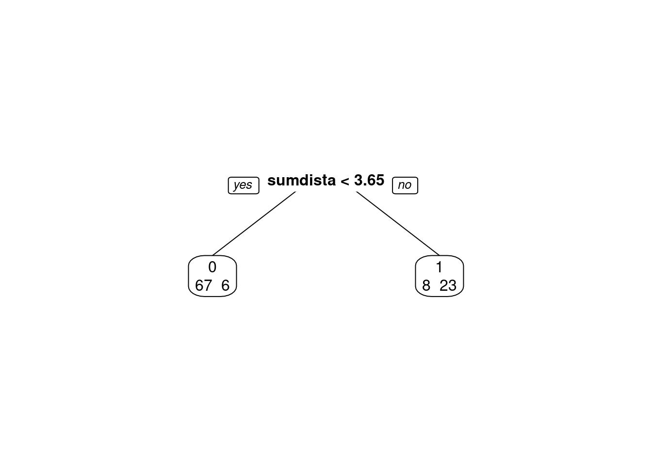
predito = predict(modArvDec01, type = "class")
cm = confusionMatrix(predito, disco$deslocamento, positive = "0")
cm## Confusion Matrix and Statistics
##
## Reference
## Prediction 0 1
## 0 67 6
## 1 8 23
##
## Accuracy : 0.8654
## 95% CI : (0.7845, 0.9244)
## No Information Rate : 0.7212
## P-Value [Acc > NIR] : 0.0003676
##
## Kappa : 0.6722
##
## Mcnemar's Test P-Value : 0.7892680
##
## Sensitivity : 0.8933
## Specificity : 0.7931
## Pos Pred Value : 0.9178
## Neg Pred Value : 0.7419
## Prevalence : 0.7212
## Detection Rate : 0.6442
## Detection Prevalence : 0.7019
## Balanced Accuracy : 0.8432
##
## 'Positive' Class : 0
## # Adiciona as métricas no df
model_eval[nrow(model_eval) + 1,] <- c("modArvDec01", "rpart", cm$overall['Accuracy'], cm$byClass['Sensitivity'], cm$byClass['Specificity'])x = 1:nrow(disco)
plot(disco$sumdistancia ~ x, col = disco$deslocamento)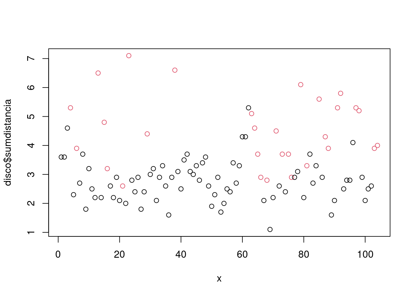
2.5.27 SVM
modSVM01 = svm(deslocamento ~ sumdistancia, data = disco, kernel = "linear")
predito = predict(modSVM01, type = "class")
cm = confusionMatrix(predito, disco$deslocamento, positive = "0")
# Adiciona as métricas no df
model_eval[nrow(model_eval) + 1,] <- c("modSVM01", "svm", cm$overall['Accuracy'], cm$byClass['Sensitivity'], cm$byClass['Specificity'])2.5.28 Rede Neural
modRedNeural01 = neuralnet(deslocamento ~ sumdistancia, data = disco, hidden = c(2,4,3))
plot(modRedNeural01)
ypred = neuralnet::compute(modRedNeural01, disco)
yhat = ypred$net.result
round(yhat)## [,1] [,2]
## [1,] 1 0
## [2,] 1 0
## [3,] 0 1
## [4,] 0 1
## [5,] 1 0
## [6,] 1 0
## [7,] 1 0
## [8,] 1 0
## [9,] 1 0
## [10,] 1 0
## [11,] 1 0
## [12,] 1 0
## [13,] 0 1
## [14,] 1 0
## [15,] 0 1
## [16,] 1 0
## [17,] 1 0
## [18,] 1 0
## [19,] 1 0
## [20,] 1 0
## [21,] 1 0
## [22,] 1 0
## [23,] 0 1
## [24,] 1 0
## [25,] 1 0
## [26,] 1 0
## [27,] 1 0
## [28,] 1 0
## [29,] 0 1
## [30,] 1 0
## [31,] 1 0
## [32,] 1 0
## [33,] 1 0
## [34,] 1 0
## [35,] 1 0
## [36,] 1 0
## [37,] 1 0
## [38,] 0 1
## [39,] 1 0
## [40,] 1 0
## [41,] 1 0
## [42,] 1 0
## [43,] 1 0
## [44,] 1 0
## [45,] 1 0
## [46,] 1 0
## [47,] 1 0
## [48,] 1 0
## [49,] 1 0
## [50,] 1 0
## [51,] 1 0
## [52,] 1 0
## [53,] 1 0
## [54,] 1 0
## [55,] 1 0
## [56,] 1 0
## [57,] 1 0
## [58,] 1 0
## [59,] 1 0
## [60,] 0 1
## [61,] 0 1
## [62,] 0 1
## [63,] 0 1
## [64,] 0 1
## [65,] 1 0
## [66,] 1 0
## [67,] 1 0
## [68,] 1 0
## [69,] 1 0
## [70,] 1 0
## [71,] 0 1
## [72,] 1 0
## [73,] 1 0
## [74,] 1 0
## [75,] 1 0
## [76,] 1 0
## [77,] 1 0
## [78,] 1 0
## [79,] 0 1
## [80,] 1 0
## [81,] 1 0
## [82,] 1 0
## [83,] 1 0
## [84,] 1 0
## [85,] 0 1
## [86,] 1 0
## [87,] 0 1
## [88,] 1 0
## [89,] 1 0
## [90,] 1 0
## [91,] 0 1
## [92,] 0 1
## [93,] 1 0
## [94,] 1 0
## [95,] 1 0
## [96,] 0 1
## [97,] 0 1
## [98,] 0 1
## [99,] 1 0
## [100,] 1 0
## [101,] 1 0
## [102,] 1 0
## [103,] 1 0
## [104,] 0 1yhat=data.frame("yhat"=ifelse(max.col(yhat[ ,1:2])==1, "0", "1"))
cm = confusionMatrix(disco$deslocamento, as.factor(yhat$yhat))
cm## Confusion Matrix and Statistics
##
## Reference
## Prediction 0 1
## 0 70 5
## 1 12 17
##
## Accuracy : 0.8365
## 95% CI : (0.7512, 0.9018)
## No Information Rate : 0.7885
## P-Value [Acc > NIR] : 0.1388
##
## Kappa : 0.5611
##
## Mcnemar's Test P-Value : 0.1456
##
## Sensitivity : 0.8537
## Specificity : 0.7727
## Pos Pred Value : 0.9333
## Neg Pred Value : 0.5862
## Prevalence : 0.7885
## Detection Rate : 0.6731
## Detection Prevalence : 0.7212
## Balanced Accuracy : 0.8132
##
## 'Positive' Class : 0
## # Adiciona as métricas no df
model_eval[nrow(model_eval) + 1,] <- c("modRedNeural01", "neuralnet", cm$overall['Accuracy'], cm$byClass['Sensitivity'], cm$byClass['Specificity'])2.5.29 KNN
modKnn1_01 = knn3(deslocamento ~ sumdistancia, data = disco, k = 1)
predito = predict(modKnn1_01, disco, type = "class")
cm = confusionMatrix(predito, disco$deslocamento, positive = "0")
cm## Confusion Matrix and Statistics
##
## Reference
## Prediction 0 1
## 0 71 11
## 1 4 18
##
## Accuracy : 0.8558
## 95% CI : (0.7733, 0.917)
## No Information Rate : 0.7212
## P-Value [Acc > NIR] : 0.0008967
##
## Kappa : 0.6127
##
## Mcnemar's Test P-Value : 0.1213353
##
## Sensitivity : 0.9467
## Specificity : 0.6207
## Pos Pred Value : 0.8659
## Neg Pred Value : 0.8182
## Prevalence : 0.7212
## Detection Rate : 0.6827
## Detection Prevalence : 0.7885
## Balanced Accuracy : 0.7837
##
## 'Positive' Class : 0
## # Adiciona as métricas no df
model_eval[nrow(model_eval) + 1,] <- c("modKnn1_01-k=1", "knn3", cm$overall['Accuracy'], cm$byClass['Sensitivity'], cm$byClass['Specificity'])k = 3
modKnn3_01 = knn3(deslocamento ~ sumdistancia, data = disco, k = 3)
predito = predict(modKnn3_01, disco, type = "class")
cm = confusionMatrix(predito, disco$deslocamento, positive = "0")
# Adiciona as métricas no df
model_eval[nrow(model_eval) + 1,] <- c("modKnn3_01-k=3", "knn3", cm$overall['Accuracy'], cm$byClass['Sensitivity'], cm$byClass['Specificity'])k = 5
modKnn5_01 = knn3(deslocamento ~ sumdistancia, data = disco, k = 5)
predito = predict(modKnn5_01, disco, type = "class")
cm = confusionMatrix(predito, disco$deslocamento, positive = "0")
cm## Confusion Matrix and Statistics
##
## Reference
## Prediction 0 1
## 0 70 7
## 1 5 22
##
## Accuracy : 0.8846
## 95% CI : (0.8071, 0.9389)
## No Information Rate : 0.7212
## P-Value [Acc > NIR] : 4.877e-05
##
## Kappa : 0.7069
##
## Mcnemar's Test P-Value : 0.7728
##
## Sensitivity : 0.9333
## Specificity : 0.7586
## Pos Pred Value : 0.9091
## Neg Pred Value : 0.8148
## Prevalence : 0.7212
## Detection Rate : 0.6731
## Detection Prevalence : 0.7404
## Balanced Accuracy : 0.8460
##
## 'Positive' Class : 0
## # Adiciona as métricas no df
model_eval[nrow(model_eval) + 1,] <- c("modKnn5_01-k=5", "knn3", cm$overall['Accuracy'], cm$byClass['Sensitivity'], cm$byClass['Specificity'])2.5.30 Avaliando os modelos
| Model | Algorithm | Accuracy | Sensitivity | Specificity |
|---|---|---|---|---|
| modLogist01 | glm | 0.173076923076923 | 0.0666666666666667 | 0.448275862068966 |
| modLogist02-LOOCV | glm | 0.826923076923077 | 0.933333333333333 | 0.551724137931034 |
| modFisher01-prior 0.5 / 0.5 | lda | 0.865384615384615 | 0.893333333333333 | 0.793103448275862 |
| modBayes01-prior 0.65 / 0.35 | lda | 0.836538461538462 | 0.933333333333333 | 0.586206896551724 |
| modNaiveBayes01 | naiveBayes | 0.826923076923077 | 0.933333333333333 | 0.551724137931034 |
| modArvDec01 | rpart | 0.865384615384615 | 0.893333333333333 | 0.793103448275862 |
| modSVM01 | svm | 0.836538461538462 | 0.946666666666667 | 0.551724137931034 |
| modRedNeural01 | neuralnet | 0.836538461538462 | 0.853658536585366 | 0.772727272727273 |
| modKnn1_01-k=1 | knn3 | 0.855769230769231 | 0.946666666666667 | 0.620689655172414 |
| modKnn3_01-k=3 | knn3 | 0.855769230769231 | 0.933333333333333 | 0.655172413793103 |
| modKnn5_01-k=5 | knn3 | 0.884615384615385 | 0.933333333333333 | 0.758620689655172 |
Os modelos tiveram performance igual ou proximo interessante o comportamento de modFisher01 com \(prior 0.5, 0.5\).
2.5.31 Agrupamento
discoS = disco[, 2:3]
d <- dist(discoS, method = "maximum")
grup = hclust(d, method = "ward.D")
plot(grup, cex = 0.6)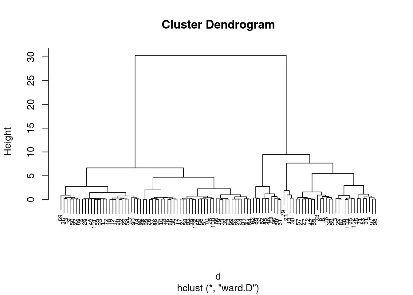
groups <- cutree(grup, k=3)table(groups, disco$deslocamento)##
## groups 0 1
## 1 10 21
## 2 58 5
## 3 7 3km1 = kmeans(discoS, 4)
p1 = fviz_cluster(km1, data=discoS,
palette = c("#2E9FDF", "#FC4E07", "#E7B800", "#E7B700"),
star.plot=FALSE,
# repel=TRUE,
ggtheme=theme_bw())
p1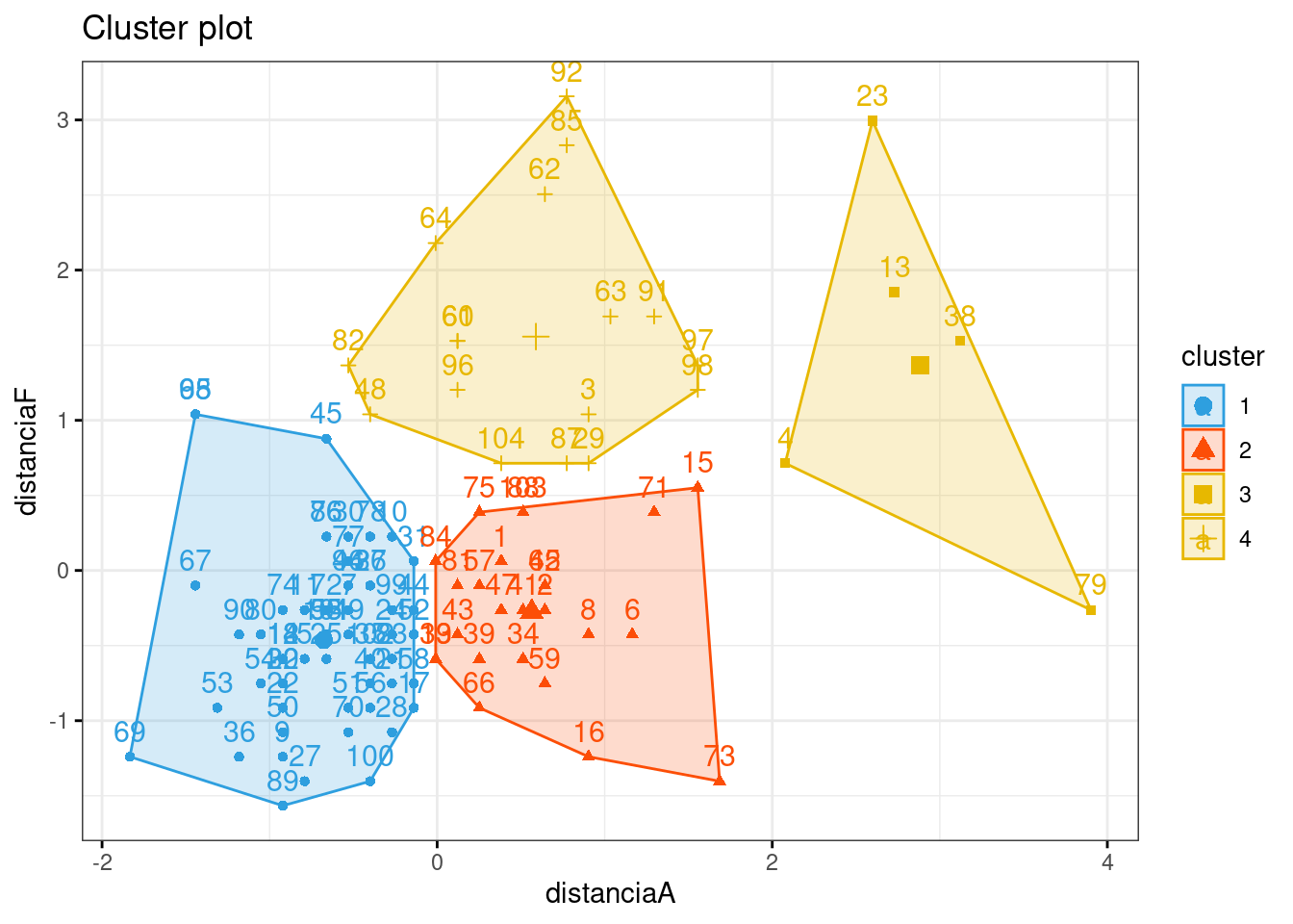
groups = km1$cluster
table(groups, disco$deslocamento)##
## groups 0 1
## 1 54 3
## 2 14 11
## 3 0 5
## 4 7 10