3 Session 2: Data management
Aim: To outline key concepts and “best practice” for working with data in R
Intended Learning Outcomes:
At the end of the session a successful student will be able to:
Compare and contrast the different types of data in R
Describe the components of “tidy data” and its advantages
Discuss the differences between the various types of joins when merging data
3.1 What will be covered today?
3.2 Data types
A key concept that is helpful to understand when you are learning R is that variables in R can be classified as a number of “types”. The various “types” dictate which functions you can apply to your date. For example, if you had a dataset with the names and telephone numbers of all learners on this course, the variable with the name will be a different type to the variable containing the telephone number.
name <- "Dave"
number <- 1234
# Check the data type using the function called class
class(name)
## [1] "character"class(number)## [1] "numeric"For a more realistic example, we can look at the africa_covid_cases object which has been assigned to the Excel file we used in Session 1. To look at the data type for a whole data frame, we use the function str
library(readxl)
library(here)
africa_covid_cases <- read_xlsx(here('data', 'africa_covid_cases.xlsx'))
str(africa_covid_cases)
## tibble [53 × 492] (S3: tbl_df/tbl/data.frame)
## $ ISO : chr [1:53] "DZA" "AGO" "BEN" "BWA" ...
## $ COUNTRY_NAME : chr [1:53] "Algeria" "Angola" "Benin" "Botswana" ...
## $ AFRICAN_REGION: chr [1:53] "Northern Africa" "Southern Africa" "Western Africa" "Southern Africa" ...
## $ 43831 : num [1:53] 0 0 0 0 0 0 0 0 0 0 ...
## $ 43832 : num [1:53] 0 0 0 0 0 0 0 0 0 0 ...
## $ 43833 : num [1:53] 0 0 0 0 0 0 0 0 0 0 ...
## $ 43834 : num [1:53] 0 0 0 0 0 0 0 0 0 0 ...
## $ 43835 : num [1:53] 0 0 0 0 0 0 0 0 0 0 ...
## $ 43836 : num [1:53] 0 0 0 0 0 0 0 0 0 0 ...
## $ 43837 : num [1:53] 0 0 0 0 0 0 0 0 0 0 ...
## $ 43838 : num [1:53] 0 0 0 0 0 0 0 0 0 0 ...
## $ 43839 : num [1:53] 0 0 0 0 0 0 0 0 0 0 ...
## $ 43840 : num [1:53] 0 0 0 0 0 0 0 0 0 0 ...
## $ 43841 : num [1:53] 0 0 0 0 0 0 0 0 0 0 ...
## $ 43842 : num [1:53] 0 0 0 0 0 0 0 0 0 0 ...
## $ 43843 : num [1:53] 0 0 0 0 0 0 0 0 0 0 ...
## $ 43844 : num [1:53] 0 0 0 0 0 0 0 0 0 0 ...
## $ 43845 : num [1:53] 0 0 0 0 0 0 0 0 0 0 ...
## $ 43846 : num [1:53] 0 0 0 0 0 0 0 0 0 0 ...
## $ 43847 : num [1:53] 0 0 0 0 0 0 0 0 0 0 ...
## $ 43848 : num [1:53] 0 0 0 0 0 0 0 0 0 0 ...
## $ 43849 : num [1:53] 0 0 0 0 0 0 0 0 0 0 ...
## $ 43850 : num [1:53] 0 0 0 0 0 0 0 0 0 0 ...
## $ 43851 : num [1:53] 0 0 0 0 0 0 0 0 0 0 ...
## $ 43852 : num [1:53] 0 0 0 0 0 0 0 0 0 0 ...
## $ 43853 : num [1:53] 0 0 0 0 0 0 0 0 0 0 ...
## $ 43854 : num [1:53] 0 0 0 0 0 0 0 0 0 0 ...
## $ 43855 : num [1:53] 0 0 0 0 0 0 0 0 0 0 ...
## $ 43856 : num [1:53] 0 0 0 0 0 0 0 0 0 0 ...
## $ 43857 : num [1:53] 0 0 0 0 0 0 0 0 0 0 ...
## $ 43858 : num [1:53] 0 0 0 0 0 0 0 0 0 0 ...
## $ 43859 : num [1:53] 0 0 0 0 0 0 0 0 0 0 ...
## $ 43860 : num [1:53] 0 0 0 0 0 0 0 0 0 0 ...
## $ 43861 : num [1:53] 0 0 0 0 0 0 0 0 0 0 ...
## $ 43862 : num [1:53] 0 0 0 0 0 0 0 0 0 0 ...
## $ 43863 : num [1:53] 0 0 0 0 0 0 0 0 0 0 ...
## $ 43864 : num [1:53] 0 0 0 0 0 0 0 0 0 0 ...
## $ 43865 : num [1:53] 0 0 0 0 0 0 0 0 0 0 ...
## $ 43866 : num [1:53] 0 0 0 0 0 0 0 0 0 0 ...
## $ 43867 : num [1:53] 0 0 0 0 0 0 0 0 0 0 ...
## $ 43868 : num [1:53] 0 0 0 0 0 0 0 0 0 0 ...
## $ 43869 : num [1:53] 0 0 0 0 0 0 0 0 0 0 ...
## $ 43870 : num [1:53] 0 0 0 0 0 0 0 0 0 0 ...
## $ 43871 : num [1:53] 0 0 0 0 0 0 0 0 0 0 ...
## $ 43872 : num [1:53] 0 0 0 0 0 0 0 0 0 0 ...
## $ 43873 : num [1:53] 0 0 0 0 0 0 0 0 0 0 ...
## $ 43874 : num [1:53] 0 0 0 0 0 0 0 0 0 0 ...
## $ 43875 : num [1:53] 0 0 0 0 0 0 0 0 0 0 ...
## $ 43876 : num [1:53] 0 0 0 0 0 0 0 0 0 0 ...
## $ 43877 : num [1:53] 0 0 0 0 0 0 0 0 0 0 ...
## $ 43878 : num [1:53] 0 0 0 0 0 0 0 0 0 0 ...
## $ 43879 : num [1:53] 0 0 0 0 0 0 0 0 0 0 ...
## $ 43880 : num [1:53] 0 0 0 0 0 0 0 0 0 0 ...
## $ 43881 : num [1:53] 0 0 0 0 0 0 0 0 0 0 ...
## $ 43882 : num [1:53] 0 0 0 0 0 0 0 0 0 0 ...
## $ 43883 : num [1:53] 0 0 0 0 0 0 0 0 0 0 ...
## $ 43884 : num [1:53] 0 0 0 0 0 0 0 0 0 0 ...
## $ 43885 : num [1:53] 0 0 0 0 0 0 0 0 0 0 ...
## $ 43886 : num [1:53] 1 0 0 0 0 0 0 0 0 0 ...
## $ 43887 : num [1:53] 0 0 0 0 0 0 0 0 0 0 ...
## $ 43888 : num [1:53] 0 0 0 0 0 0 0 0 0 0 ...
## $ 43889 : num [1:53] 0 0 0 0 0 0 0 0 0 0 ...
## $ 43890 : num [1:53] 0 0 0 0 0 0 0 0 0 0 ...
## $ 43891 : num [1:53] 2 0 0 0 0 0 0 0 0 0 ...
## $ 43892 : num [1:53] 2 0 0 0 0 0 0 0 0 0 ...
## $ 43893 : num [1:53] 0 0 0 0 0 0 0 0 0 0 ...
## $ 43894 : num [1:53] 7 0 0 0 0 0 0 0 0 0 ...
## $ 43895 : num [1:53] 5 0 0 0 0 0 0 0 0 0 ...
## $ 43896 : num [1:53] 0 0 0 0 0 0 1 0 0 0 ...
## $ 43897 : num [1:53] 2 0 0 0 0 0 0 0 0 0 ...
## $ 43898 : num [1:53] 1 0 0 0 0 0 1 0 0 0 ...
## $ 43899 : num [1:53] 0 0 0 0 2 0 0 0 0 0 ...
## $ 43900 : num [1:53] 0 0 0 0 0 0 0 0 0 0 ...
## $ 43901 : num [1:53] 0 0 0 0 0 0 0 0 0 0 ...
## $ 43902 : num [1:53] 5 0 0 0 0 0 0 0 0 0 ...
## $ 43903 : num [1:53] 1 0 0 0 1 0 0 0 0 0 ...
## $ 43904 : num [1:53] 11 0 0 0 4 0 2 1 0 0 ...
## $ 43905 : num [1:53] 17 0 0 0 8 0 1 0 0 0 ...
## $ 43906 : num [1:53] 0 0 1 0 5 0 0 0 0 0 ...
## $ 43907 : num [1:53] 6 0 1 0 7 0 5 0 0 0 ...
## $ 43908 : num [1:53] 12 0 0 0 6 0 0 0 0 0 ...
## $ 43909 : num [1:53] 18 0 0 0 7 0 0 2 1 0 ...
## $ 43910 : num [1:53] 12 0 0 0 24 0 17 0 0 0 ...
## $ 43911 : num [1:53] 37 2 0 0 11 0 13 0 0 0 ...
## $ 43912 : num [1:53] 62 0 3 0 24 0 0 1 0 0 ...
## $ 43913 : num [1:53] 29 1 0 0 15 0 16 0 0 0 ...
## $ 43914 : num [1:53] 34 0 0 0 32 0 10 1 2 0 ...
## $ 43915 : num [1:53] 38 0 0 0 6 0 0 0 0 0 ...
## $ 43916 : num [1:53] 65 1 0 0 28 0 22 0 2 0 ...
## $ 43917 : num [1:53] 42 0 0 0 27 0 4 1 0 0 ...
## $ 43918 : num [1:53] 45 1 1 0 15 0 7 0 0 0 ...
## $ 43919 : num [1:53] 57 2 0 0 24 0 40 0 0 0 ...
## $ 43920 : num [1:53] 73 0 0 3 15 0 3 0 2 0 ...
## $ 43921 : num [1:53] 132 0 0 1 21 2 51 0 0 0 ...
## $ 43922 : num [1:53] 131 0 7 0 6 0 40 2 0 0 ...
## $ 43923 : num [1:53] 139 1 0 0 14 1 73 1 0 0 ...
## $ 43924 : num [1:53] 185 0 3 0 16 0 203 0 0 0 ...
## $ 43925 : num [1:53] 80 2 0 0 27 0 0 0 0 0 ...
## $ 43926 : num [1:53] 69 4 6 2 19 0 141 0 0 0 ...
## [list output truncated]The first 3 columns are of the class “chr” which is short for character. These are often known as “strings”. We can see the remaining variables are of the class “num”, which means that R has identified these variables as numbers.
Depending on the data type, we can apply different functions. For example, we can get the average of the first numeric column by typing.
mean(africa_covid_cases$`43831`)## [1] 0However, we cannot get the mean value of the character columns because they do not contain data that has been identified by R as a number.
mean(africa_covid_cases$ISO)## Warning in mean.default(africa_covid_cases$ISO): argument is not numeric or
## logical: returning NA## [1] NA3.3 Working with data
In the africa_covid_cases object, there are 53 obs (observations) of 492 variables.
So what does this mean?
We can look at our data to get more information
africa_covid_cases## # A tibble: 53 x 492
## ISO COUNTRY_NAME AFRICAN_REGION `43831` `43832` `43833` `43834` `43835`
## <chr> <chr> <chr> <dbl> <dbl> <dbl> <dbl> <dbl>
## 1 DZA Algeria Northern Afri… 0 0 0 0 0
## 2 AGO Angola Southern Afri… 0 0 0 0 0
## 3 BEN Benin Western Africa 0 0 0 0 0
## 4 BWA Botswana Southern Afri… 0 0 0 0 0
## 5 BFA Burkina Faso Western Africa 0 0 0 0 0
## 6 BDI Burundi Central Africa 0 0 0 0 0
## 7 CMR Cameroon Central Africa 0 0 0 0 0
## 8 CAR Central African… Central Africa 0 0 0 0 0
## 9 TCD Chad Central Africa 0 0 0 0 0
## 10 COM Comoros Eastern Africa 0 0 0 0 0
## # … with 43 more rows, and 484 more variables: 43836 <dbl>, 43837 <dbl>,
## # 43838 <dbl>, 43839 <dbl>, 43840 <dbl>, 43841 <dbl>, 43842 <dbl>,
## # 43843 <dbl>, 43844 <dbl>, 43845 <dbl>, 43846 <dbl>, 43847 <dbl>,
## # 43848 <dbl>, 43849 <dbl>, 43850 <dbl>, 43851 <dbl>, 43852 <dbl>,
## # 43853 <dbl>, 43854 <dbl>, 43855 <dbl>, 43856 <dbl>, 43857 <dbl>,
## # 43858 <dbl>, 43859 <dbl>, 43860 <dbl>, 43861 <dbl>, 43862 <dbl>,
## # 43863 <dbl>, 43864 <dbl>, 43865 <dbl>, 43866 <dbl>, 43867 <dbl>,
## # 43868 <dbl>, 43869 <dbl>, 43870 <dbl>, 43871 <dbl>, 43872 <dbl>,
## # 43873 <dbl>, 43874 <dbl>, 43875 <dbl>, 43876 <dbl>, 43877 <dbl>,
## # 43878 <dbl>, 43879 <dbl>, 43880 <dbl>, 43881 <dbl>, 43882 <dbl>,
## # 43883 <dbl>, 43884 <dbl>, 43885 <dbl>, 43886 <dbl>, 43887 <dbl>,
## # 43888 <dbl>, 43889 <dbl>, 43890 <dbl>, 43891 <dbl>, 43892 <dbl>,
## # 43893 <dbl>, 43894 <dbl>, 43895 <dbl>, 43896 <dbl>, 43897 <dbl>,
## # 43898 <dbl>, 43899 <dbl>, 43900 <dbl>, 43901 <dbl>, 43902 <dbl>,
## # 43903 <dbl>, 43904 <dbl>, 43905 <dbl>, 43906 <dbl>, 43907 <dbl>,
## # 43908 <dbl>, 43909 <dbl>, 43910 <dbl>, 43911 <dbl>, 43912 <dbl>,
## # 43913 <dbl>, 43914 <dbl>, 43915 <dbl>, 43916 <dbl>, 43917 <dbl>,
## # 43918 <dbl>, 43919 <dbl>, 43920 <dbl>, 43921 <dbl>, 43922 <dbl>,
## # 43923 <dbl>, 43924 <dbl>, 43925 <dbl>, 43926 <dbl>, 43927 <dbl>,
## # 43928 <dbl>, 43929 <dbl>, 43930 <dbl>, 43931 <dbl>, 43932 <dbl>,
## # 43933 <dbl>, 43934 <dbl>, 43935 <dbl>, …ISO - 3 letter code assigned to each country
COUNTRY_NAME - Name of the country
AFRICAN_REGION - African region
43831, 43832, 43833 - This looks like a date format used by Excel. It is the number of days since January 1, 1970.
3.3.1 Looking at your data
Show the first 5 rows of the data frame.
The function head tells R that we want to see the first few rows and n= specifies how many rows we want to see.
head(africa_covid_cases, n=5)## # A tibble: 5 x 492
## ISO COUNTRY_NAME AFRICAN_REGION `43831` `43832` `43833` `43834` `43835`
## <chr> <chr> <chr> <dbl> <dbl> <dbl> <dbl> <dbl>
## 1 DZA Algeria Northern Africa 0 0 0 0 0
## 2 AGO Angola Southern Africa 0 0 0 0 0
## 3 BEN Benin Western Africa 0 0 0 0 0
## 4 BWA Botswana Southern Africa 0 0 0 0 0
## 5 BFA Burkina Faso Western Africa 0 0 0 0 0
## # … with 484 more variables: 43836 <dbl>, 43837 <dbl>, 43838 <dbl>,
## # 43839 <dbl>, 43840 <dbl>, 43841 <dbl>, 43842 <dbl>, 43843 <dbl>,
## # 43844 <dbl>, 43845 <dbl>, 43846 <dbl>, 43847 <dbl>, 43848 <dbl>,
## # 43849 <dbl>, 43850 <dbl>, 43851 <dbl>, 43852 <dbl>, 43853 <dbl>,
## # 43854 <dbl>, 43855 <dbl>, 43856 <dbl>, 43857 <dbl>, 43858 <dbl>,
## # 43859 <dbl>, 43860 <dbl>, 43861 <dbl>, 43862 <dbl>, 43863 <dbl>,
## # 43864 <dbl>, 43865 <dbl>, 43866 <dbl>, 43867 <dbl>, 43868 <dbl>,
## # 43869 <dbl>, 43870 <dbl>, 43871 <dbl>, 43872 <dbl>, 43873 <dbl>,
## # 43874 <dbl>, 43875 <dbl>, 43876 <dbl>, 43877 <dbl>, 43878 <dbl>,
## # 43879 <dbl>, 43880 <dbl>, 43881 <dbl>, 43882 <dbl>, 43883 <dbl>,
## # 43884 <dbl>, 43885 <dbl>, 43886 <dbl>, 43887 <dbl>, 43888 <dbl>,
## # 43889 <dbl>, 43890 <dbl>, 43891 <dbl>, 43892 <dbl>, 43893 <dbl>,
## # 43894 <dbl>, 43895 <dbl>, 43896 <dbl>, 43897 <dbl>, 43898 <dbl>,
## # 43899 <dbl>, 43900 <dbl>, 43901 <dbl>, 43902 <dbl>, 43903 <dbl>,
## # 43904 <dbl>, 43905 <dbl>, 43906 <dbl>, 43907 <dbl>, 43908 <dbl>,
## # 43909 <dbl>, 43910 <dbl>, 43911 <dbl>, 43912 <dbl>, 43913 <dbl>,
## # 43914 <dbl>, 43915 <dbl>, 43916 <dbl>, 43917 <dbl>, 43918 <dbl>,
## # 43919 <dbl>, 43920 <dbl>, 43921 <dbl>, 43922 <dbl>, 43923 <dbl>,
## # 43924 <dbl>, 43925 <dbl>, 43926 <dbl>, 43927 <dbl>, 43928 <dbl>,
## # 43929 <dbl>, 43930 <dbl>, 43931 <dbl>, 43932 <dbl>, 43933 <dbl>,
## # 43934 <dbl>, 43935 <dbl>, …Show the last 7 rows of the data frame.
tail(africa_covid_cases, n=7)## # A tibble: 7 x 492
## ISO COUNTRY_NAME AFRICAN_REGION `43831` `43832` `43833` `43834` `43835`
## <chr> <chr> <chr> <dbl> <dbl> <dbl> <dbl> <dbl>
## 1 SDN Sudan Eastern Africa 0 0 0 0 0
## 2 TZA Tanzania Eastern Africa 0 0 0 0 0
## 3 TGO Togo Western Africa 0 0 0 0 0
## 4 TUN Tunisia Northern Africa 0 0 0 0 0
## 5 UGA Uganda Eastern Africa 0 0 0 0 0
## 6 ZMB Zambia Southern Africa 0 0 0 0 0
## 7 ZWE Zimbabwe Southern Africa 0 0 0 0 0
## # … with 484 more variables: 43836 <dbl>, 43837 <dbl>, 43838 <dbl>,
## # 43839 <dbl>, 43840 <dbl>, 43841 <dbl>, 43842 <dbl>, 43843 <dbl>,
## # 43844 <dbl>, 43845 <dbl>, 43846 <dbl>, 43847 <dbl>, 43848 <dbl>,
## # 43849 <dbl>, 43850 <dbl>, 43851 <dbl>, 43852 <dbl>, 43853 <dbl>,
## # 43854 <dbl>, 43855 <dbl>, 43856 <dbl>, 43857 <dbl>, 43858 <dbl>,
## # 43859 <dbl>, 43860 <dbl>, 43861 <dbl>, 43862 <dbl>, 43863 <dbl>,
## # 43864 <dbl>, 43865 <dbl>, 43866 <dbl>, 43867 <dbl>, 43868 <dbl>,
## # 43869 <dbl>, 43870 <dbl>, 43871 <dbl>, 43872 <dbl>, 43873 <dbl>,
## # 43874 <dbl>, 43875 <dbl>, 43876 <dbl>, 43877 <dbl>, 43878 <dbl>,
## # 43879 <dbl>, 43880 <dbl>, 43881 <dbl>, 43882 <dbl>, 43883 <dbl>,
## # 43884 <dbl>, 43885 <dbl>, 43886 <dbl>, 43887 <dbl>, 43888 <dbl>,
## # 43889 <dbl>, 43890 <dbl>, 43891 <dbl>, 43892 <dbl>, 43893 <dbl>,
## # 43894 <dbl>, 43895 <dbl>, 43896 <dbl>, 43897 <dbl>, 43898 <dbl>,
## # 43899 <dbl>, 43900 <dbl>, 43901 <dbl>, 43902 <dbl>, 43903 <dbl>,
## # 43904 <dbl>, 43905 <dbl>, 43906 <dbl>, 43907 <dbl>, 43908 <dbl>,
## # 43909 <dbl>, 43910 <dbl>, 43911 <dbl>, 43912 <dbl>, 43913 <dbl>,
## # 43914 <dbl>, 43915 <dbl>, 43916 <dbl>, 43917 <dbl>, 43918 <dbl>,
## # 43919 <dbl>, 43920 <dbl>, 43921 <dbl>, 43922 <dbl>, 43923 <dbl>,
## # 43924 <dbl>, 43925 <dbl>, 43926 <dbl>, 43927 <dbl>, 43928 <dbl>,
## # 43929 <dbl>, 43930 <dbl>, 43931 <dbl>, 43932 <dbl>, 43933 <dbl>,
## # 43934 <dbl>, 43935 <dbl>, …How many unique countries are in the data?
unique(africa_covid_cases$COUNTRY_NAME)## [1] "Algeria" "Angola"
## [3] "Benin" "Botswana"
## [5] "Burkina Faso" "Burundi"
## [7] "Cameroon" "Central African Republic"
## [9] "Chad" "Comoros"
## [11] "Congo" "Cote d'Ivoire"
## [13] "Democratic Republic of the Congo" "Djibouti"
## [15] "Egypt" "Equatorial Guinea"
## [17] "Eritrea" "Eswatini"
## [19] "Ethiopia" "Gabon"
## [21] "Gambia" "Ghana"
## [23] "Guinea" "Guinea-Bissau"
## [25] "Kenya" "Lesotho"
## [27] "Liberia" "Libya"
## [29] "Madagascar" "Malawi"
## [31] "Mali" "Mauritania"
## [33] "Mauritius" "Mayotte"
## [35] "Morocco" "Mozambique"
## [37] "Namibia" "Niger"
## [39] "Nigeria" "Rwanda"
## [41] "Sao Tome and Principe" "Senegal"
## [43] "Sierra Leone" "Somalia"
## [45] "South Africa" "South Sudan"
## [47] "Sudan" "Tanzania"
## [49] "Togo" "Tunisia"
## [51] "Uganda" "Zambia"
## [53] "Zimbabwe"There are 53 unique country values. This is helpful as there are also 53 rows so we can say that each row represents a country. We can assign the list of unique countries to an object for future reference
country_list <- unique(africa_covid_cases$COUNTRY_NAME)3.3.2 Looking at one variable
In the previous step, the following command was used
unique(africa_covid_cases$COUNTRY_NAME)
What does “$” do in R?
It allows us to look at a specific variable within the dataset
unique(africa_covid_cases$AFRICAN_REGION)## [1] "Northern Africa" "Southern Africa" "Western Africa" "Central Africa"
## [5] "Eastern Africa"And again we can assign this result to an object.
region_list <- unique(africa_covid_cases$AFRICAN_REGION)3.4 The tidyverse
When using R, there are many approaches you can use to reach the same result.
There are thousands of packages with many functions and sometimes these packages can overlap.
This can be confusing when you are starting to learn R.
There is a collection of packages with many of the most commonly used packages, and this is called the tidyverse.
tidyverse::tidyverse_packages()## [1] "broom" "cli" "crayon" "dbplyr"
## [5] "dplyr" "dtplyr" "forcats" "googledrive"
## [9] "googlesheets4" "ggplot2" "haven" "hms"
## [13] "httr" "jsonlite" "lubridate" "magrittr"
## [17] "modelr" "pillar" "purrr" "readr"
## [21] "readxl" "reprex" "rlang" "rstudioapi"
## [25] "rvest" "stringr" "tibble" "tidyr"
## [29] "xml2" "tidyverse"We will use functions from some of these packages over the next few sessions.
3.4.1 Tidy data
The key concept when working with packages from the tidyverse is the concept of “tidy data”.
R for Epidemiologist handbook 4.1 From Excel - Tidy data
Principles of “tidy data”:
- Each variable must have its own column.
- Each observation must have its own row.
- Each value must have its own cell.
Functions from the tidyverse packages are set up to work with tidy data. If your data are not tidy, then you will have to restructure the data to a tidy format. Restructuring can take a lot of time if the data are stored in Excel spreadsheets with a lot of formatting/merged columns.
3.4.2 Checking if data are tidy
In a previous step, we imported COVID case data from an Excel spreadsheet. But how do we know if the data are “tidy”
Remember there are 3 principles:
- Each variable must have its own column.
- Each observation must have its own row.
- Each value must have its own cell.
head(africa_covid_cases, n=3)## # A tibble: 3 x 492
## ISO COUNTRY_NAME AFRICAN_REGION `43831` `43832` `43833` `43834` `43835`
## <chr> <chr> <chr> <dbl> <dbl> <dbl> <dbl> <dbl>
## 1 DZA Algeria Northern Africa 0 0 0 0 0
## 2 AGO Angola Southern Africa 0 0 0 0 0
## 3 BEN Benin Western Africa 0 0 0 0 0
## # … with 484 more variables: 43836 <dbl>, 43837 <dbl>, 43838 <dbl>,
## # 43839 <dbl>, 43840 <dbl>, 43841 <dbl>, 43842 <dbl>, 43843 <dbl>,
## # 43844 <dbl>, 43845 <dbl>, 43846 <dbl>, 43847 <dbl>, 43848 <dbl>,
## # 43849 <dbl>, 43850 <dbl>, 43851 <dbl>, 43852 <dbl>, 43853 <dbl>,
## # 43854 <dbl>, 43855 <dbl>, 43856 <dbl>, 43857 <dbl>, 43858 <dbl>,
## # 43859 <dbl>, 43860 <dbl>, 43861 <dbl>, 43862 <dbl>, 43863 <dbl>,
## # 43864 <dbl>, 43865 <dbl>, 43866 <dbl>, 43867 <dbl>, 43868 <dbl>,
## # 43869 <dbl>, 43870 <dbl>, 43871 <dbl>, 43872 <dbl>, 43873 <dbl>,
## # 43874 <dbl>, 43875 <dbl>, 43876 <dbl>, 43877 <dbl>, 43878 <dbl>,
## # 43879 <dbl>, 43880 <dbl>, 43881 <dbl>, 43882 <dbl>, 43883 <dbl>,
## # 43884 <dbl>, 43885 <dbl>, 43886 <dbl>, 43887 <dbl>, 43888 <dbl>,
## # 43889 <dbl>, 43890 <dbl>, 43891 <dbl>, 43892 <dbl>, 43893 <dbl>,
## # 43894 <dbl>, 43895 <dbl>, 43896 <dbl>, 43897 <dbl>, 43898 <dbl>,
## # 43899 <dbl>, 43900 <dbl>, 43901 <dbl>, 43902 <dbl>, 43903 <dbl>,
## # 43904 <dbl>, 43905 <dbl>, 43906 <dbl>, 43907 <dbl>, 43908 <dbl>,
## # 43909 <dbl>, 43910 <dbl>, 43911 <dbl>, 43912 <dbl>, 43913 <dbl>,
## # 43914 <dbl>, 43915 <dbl>, 43916 <dbl>, 43917 <dbl>, 43918 <dbl>,
## # 43919 <dbl>, 43920 <dbl>, 43921 <dbl>, 43922 <dbl>, 43923 <dbl>,
## # 43924 <dbl>, 43925 <dbl>, 43926 <dbl>, 43927 <dbl>, 43928 <dbl>,
## # 43929 <dbl>, 43930 <dbl>, 43931 <dbl>, 43932 <dbl>, 43933 <dbl>,
## # 43934 <dbl>, 43935 <dbl>, …So are the data “tidy”?
The data from the spreadsheet are not “tidy”.
The columns “43831, 43832, 43833…” represent different dates. Therefore, this does meet the second argument of “tidy data” - “Each observation must have its own row”.But we can reformat the data to make it “tidy” using functions from the packages included in the tidyverse
Remember, first we must install the packages from the tidyverse
install.packages("tidyverse")
3.4.3 Tidying data
Now that the tidyverse has been installed, we can use the functions from the packages to “tidy” the data.
One package which is very helpful for this is called tidyr. Instead of loading individual packages, we can load the core tidyverse packages with one command.
library(tidyverse)## ── Attaching packages ─────────────────────────────────────── tidyverse 1.3.1 ──## ✓ ggplot2 3.3.4 ✓ purrr 0.3.4
## ✓ tibble 3.1.2 ✓ dplyr 1.0.7
## ✓ tidyr 1.1.3 ✓ stringr 1.4.0
## ✓ readr 1.4.0 ✓ forcats 0.5.1## ── Conflicts ────────────────────────────────────────── tidyverse_conflicts() ──
## x dplyr::filter() masks stats::filter()
## x dplyr::lag() masks stats::lag()The core packages contain powerful functions we can use to process, analyse and visualise data.
Remember to look at the documentation for a package type “?[name of package]”
Example -
?tidyr
To look at the functions within a package, type [name of package]::
Example
tidyr::
To reformat the data to a tidy format, we need to transform the data from wide to long.
The Epidemiologist R handbook has an excellent section describing how to do this
12 - Pivoting data
3.4.4 Wide to long
africa_covid_cases_long <-
  africa_covid_cases %>% #tell R to use this dataset
  pivot_longer(cols = 4:492,#select the columns you want
               names_to = "excel_date", #name the new date column
               values_to = "cases") #name the new cases column
Transforming data from wide to long usually requires a few attempts to ensure you have achieved the correct outcome!
head(africa_covid_cases_long, n=3)## # A tibble: 3 x 5
## ISO COUNTRY_NAME AFRICAN_REGION excel_date cases
## <chr> <chr> <chr> <chr> <dbl>
## 1 DZA Algeria Northern Africa 43831 0
## 2 DZA Algeria Northern Africa 43832 0
## 3 DZA Algeria Northern Africa 43833 0This looks correct!
3.4.5 Piping
When we created the object africa_covid_cases_long, you may have noticed this %>%
This is called a pipe and more information can be found in the Epidemiologist R handbook: 3.11 Piping
Pipes are used to link together multiple functions that you have instructed R to apply to a data frame. You can add comments to code to show other people (and remind yourself!) why you wrote the code in a particular way. Functions are carried out in the order they are linked to one another using pipes.
The example applies the concept of piping to a recipe for baking a cake.
# A fake example of how to bake a cake using piping syntax

cake <- flour %>%       # to define cake, start with flour, and then...
  add(eggs) %>%   # add eggs
  add(oil) %>%    # add oil
  add(water) %>%  # add water
  mix_together(         # mix together
    utensil = spoon,
    minutes = 2) %>%
  bake(degrees = 350,   # bake
       system = "fahrenheit",
       minutes = 35) %>%
  let_cool()            # let it cool down
3.4.6 Merging
So far we have been working through examples using one dataset which we imported from an Excel file. Often it is necessary to import additional datasets and merge the two datasets into one. The tidyverse makes this process straightforward but before working through an example, we will briefly discuss the different types of merges you can do in R.
3.4.6.1 Types of joins
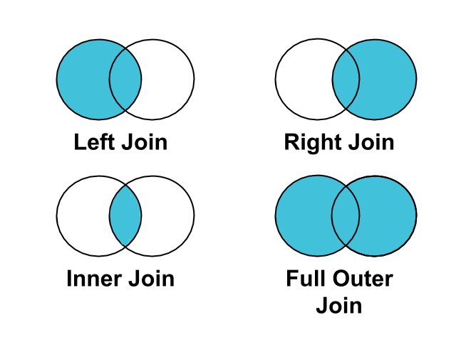
This diagram shows some of the most common types of join you will encounter while working with data. When joining data, you need to tell R which column is in dataset A that can link to dataset B. The type of join depends on what relationship you are trying to achieve.
3.4.6.2 Example of a join
In africa_covid_cases_long we have information about the number of confirmed COVID-19 cases for countries in Africa. To compare the data between countries it would be helpful to have population data for each country. This will allow us to estimate the total COVID-19 cases per 100,000 people.
#Import population dataset
population_data <- read.csv(here('data','world_population_2021.csv'))
summary(population_data)
## Location PopTotal PopDensity
## Length:285 Min. : 1 Min. : 0.139
## Class :character 1st Qu.: 705 1st Qu.: 33.018
## Mode :character Median : 9437 Median : 82.565
## Mean : 259672 Mean : 407.795
## 3rd Qu.: 47082 3rd Qu.: 208.593
## Max. :7876435 Max. :26517.450head(population_data)## Location PopTotal PopDensity
## 1 Afghanistan 39943.186 61.182
## 2 Africa 1374661.367 46.365
## 3 Albania 2871.801 104.810
## 4 Algeria 44669.558 18.755
## 5 American Samoa 55.137 275.685
## 6 Andorra 77.406 164.694It looks like the dataset has one row for each country/region. There are 3 columns
names(population_data)## [1] "Location" "PopTotal" "PopDensity"The column “Location” will be used to join the population data to the africa_covid_long dataset. We can check the names of the columns in africa_covid_long to see what variable we can join on.
names(africa_covid_cases_long)## [1] "ISO" "COUNTRY_NAME" "AFRICAN_REGION" "excel_date"
## [5] "cases"“COUNTRY_NAME” will be used for the join. You will have noticed that the two datasets we are trying to join have different column names. Unlike other statistical programs (such as Stata), this is not a problem. We can use functions from the dplyr package to join the data.
merged_data_left_join <- left_join(africa_covid_cases_long,
                         population_data,
                         by=c("COUNTRY_NAME"="Location"))
str(merged_data_left_join)
## tibble [25,917 × 7] (S3: tbl_df/tbl/data.frame)
## $ ISO : chr [1:25917] "DZA" "DZA" "DZA" "DZA" ...
## $ COUNTRY_NAME : chr [1:25917] "Algeria" "Algeria" "Algeria" "Algeria" ...
## $ AFRICAN_REGION: chr [1:25917] "Northern Africa" "Northern Africa" "Northern Africa" "Northern Africa" ...
## $ excel_date : chr [1:25917] "43831" "43832" "43833" "43834" ...
## $ cases : num [1:25917] 0 0 0 0 0 0 0 0 0 0 ...
## $ PopTotal : num [1:25917] 44670 44670 44670 44670 44670 ...
## $ PopDensity : num [1:25917] 18.8 18.8 18.8 18.8 18.8 ...The merge has successfully joined the COVID data and the population data. We can change the type of join to see how this changes the results.
merged_data_inner_join <- inner_join(africa_covid_cases_long,
                         population_data,
                         by=c("COUNTRY_NAME"="Location"))
str(merged_data_inner_join)
## tibble [24,939 × 7] (S3: tbl_df/tbl/data.frame)
## $ ISO : chr [1:24939] "DZA" "DZA" "DZA" "DZA" ...
## $ COUNTRY_NAME : chr [1:24939] "Algeria" "Algeria" "Algeria" "Algeria" ...
## $ AFRICAN_REGION: chr [1:24939] "Northern Africa" "Northern Africa" "Northern Africa" "Northern Africa" ...
## $ excel_date : chr [1:24939] "43831" "43832" "43833" "43834" ...
## $ cases : num [1:24939] 0 0 0 0 0 0 0 0 0 0 ...
## $ PopTotal : num [1:24939] 44670 44670 44670 44670 44670 ...
## $ PopDensity : num [1:24939] 18.8 18.8 18.8 18.8 18.8 ...merged_data_right_join <- right_join(africa_covid_cases_long,
population_data,
by=c("COUNTRY_NAME"="Location"))
str(merged_data_right_join)## tibble [25,173 × 7] (S3: tbl_df/tbl/data.frame)
## $ ISO : chr [1:25173] "DZA" "DZA" "DZA" "DZA" ...
## $ COUNTRY_NAME : chr [1:25173] "Algeria" "Algeria" "Algeria" "Algeria" ...
## $ AFRICAN_REGION: chr [1:25173] "Northern Africa" "Northern Africa" "Northern Africa" "Northern Africa" ...
## $ excel_date : chr [1:25173] "43831" "43832" "43833" "43834" ...
## $ cases : num [1:25173] 0 0 0 0 0 0 0 0 0 0 ...
## $ PopTotal : num [1:25173] 44670 44670 44670 44670 44670 ...
## $ PopDensity : num [1:25173] 18.8 18.8 18.8 18.8 18.8 ...This is an important concept to understand. If the join is not doing what you want it to do, your analysis could be wrong!
Additional examples can be found in the Epidemiologist R handbook 14.2 dplyr joins
3.5 Working with dates
To add to the confusion, Excel has 2 additional date systems:
1900 date system
1904 date system
In the data set we are using, the dates are in this format:
head(africa_covid_cases_long$excel_date)## [1] "43831" "43832" "43833" "43834" "43835" "43836"We can use a function from another package to convert this to a standard date format.
install.packages("janitor")library(janitor)##
## Attaching package: 'janitor'## The following objects are masked from 'package:stats':
##
## chisq.test, fisher.testThe package janitor has many helpful functions for cleaning data. For example, the function excel_numeric_to_date can be used to convert the Excel dates to a more understandable format.
africa_covid_cases_long <- africa_covid_cases_long %>%
  mutate(date_format=excel_numeric_to_date(as.numeric(excel_date)))

head(africa_covid_cases_long$date_format)
## [1] "2020-01-01" "2020-01-02" "2020-01-03" "2020-01-04" "2020-01-05"
## [6] "2020-01-06"The new variable created “date_format” is in the format YEAR-MONTH-DATE.
We can also check if the values in the new variable look correct
min(africa_covid_cases_long$date_format) #minimum date## [1] "2020-01-01"max(africa_covid_cases_long$date_format) #maximum date## [1] "2021-05-03"We know this is a data set of COVID cases so the date range (from the start of 2020 through to May of 2021) looks to be correct.
3.6 Keeping your workspace clean
All of the objects you have created so far will be visible in the top right corner of RStudio. As you proceed through your analysis this can become cluttered making it difficult to ensure you are using the correct dataset for your analysis. To remove individual objects, type rm(object name)where object name is the object you want to remove from your workspace.
#remove object called population_data
rm(population_data)
#remove all objects except africa_covid_cases_long and merged_data_right_join
rm(list=ls()[! ls() %in% c("africa_covid_cases_long","merged_data_right_join")])
#remove all objects except africa_covid_cases_long
rm(list=setdiff(ls(), "africa_covid_cases_long"))
write.csv(africa_covid_cases_long, here('data', 'africa_covid_cases_long.csv'))
When using the rm function to remove objects, you are not deleting data from your folders. You are only deleting objects from your RStudio workspace. Make sure the data you are working on is stored in a secure location so that if you accidentally save over the raw data, you can get the data back!
3.7 Useful resources
Epidemiologist R handbook
Basics
- 3: R Basics
- 4: Transition to R
Data management
12: Pivoting data
14: Joining data