Chapter 4 Objects, functions, and packages
Now that we have a basic understanding about what it means to run code and what scripts are, let us introduce the fundamental workhorses of R. Objects, functions, and packages.
4.1 Objects
An object is simply something, anything, that we want R to store so that we can access it. It can be anything from a single value, to a collection of values, to a data set, a function, or even a list of other objects. The only limit for objects are basically that each object needs to have a unique name, which is used to call the object.
To create an object we use the so called assignment operator, which is simply this arrow: <- where we put the name of the object that we want to create on the left hand side of the arrow, and the object itself on the right hand side of the arrow. The name of the object cannot start with a number and is not allowed to contain spaces, or a number of special signs such as +, -, :, $ and others. A good convention to get around the fact that you are not allowed to use spaces in names is to use either snake_case, in which you separate words with underscores _ and which is the convention I will follow in this book, CamelCase, in which you put a capital letter as the first letter in each word, or period.case, in which you put periods between words. Another good convention is to name your objects descriptively so that you remember what they refer to. Using what we know, we can now create our first object by running the following code. Remember that you should always keep track of what you are doing, so you should write the code in the script and then running it by highlighting it and pressing Ctrl+Enter.
my_first_object <- 32If you look at the environment pane, you will now see that an object appeared in our environment, and that object is called ‘my_first_object.’ The name here is arbitrary, and we could have named it anything (as long as it does not contain spaces or begin with a number). We can now call our object by simply writing the object name and running the code:
> my_first_object
[1] 32
As you can see, R simply fetches the object and prints it out. As ‘my_first_object’ is a number, we can treat it as any other number and perform mathematical operation on it, such as running my_first_object*2+4 which would yield:
> my_first_object*2+4
[1] 68
We can also define a second object, and assign a number to it. For instance
another_object <- 21and then we can call both objects to for instance add them together
> my_first_object + another_object
[1] 53
If we then want to replace either of the variables, we can simply overwrite them by creating a new object with the same name. For instance by running
another_object <- 15Then when we add the objects together we will see that
> my_first_object + another_object
[1] 47
So, how is this useful in practice? Well, let’s say that you are interested in the number of people who have voted for a certain party in an election, but you only have access to the total number of people who voted and the vote shares of each party. We could then for instance run
# Calculating the number of votes for a specific party

voting_pop <- 9321800 # The number of people who cast their votes
vote_share <- 0.52 # The vote share of the party of interest

number_of_votes <- voting_pop*vote_share # Number of votes cast for the party
If we then want to investigate the number of votes for another party, all we need to do is simply change the value for the object vote_share to the vote share of the other party we are interested in knowing the number of votes for. If we are doing many calculations using a single object, we can save a lot of time by structuring our calculations in a script like above.
Another alternative if we want to investigate how many people voted for a number of different parties is to create a vector of values containing the vote shares of each party we are interested in. A vector is simply a collection of values, and are created with the function c(). We will talk more about functions very shortly, but for now it is enough to know that c() is a function which takes multiple values, separated by commas, and combines them into one object. Let us run
vote_shares <- c(0.52,0.44,0.04) # Vote shares of all parties of interestWe can then access each individual values in the vote_shares vector by using hard brackets [] with the position inside the brackets. You can try this by running
vote_shares[1]
vote_shares[2]
vote_shares[3]
Similarly we can obtain the number of people voting for each party by multiplying the vote shares from each party with the total number of voters
voting_pop*vote_shares[1] # Number of people who voted for the first party
voting_pop*vote_shares[2] # Number of people who voted for the second party
voting_pop*vote_shares[3] # Number of people who voted for the third party
4.2 Functions
While objects are everything that we store in R, functions are everything that we do in R. Functions make the calculations, and functions are what makes R a statistical programming language. A function is a piece of code that takes some object or objects and performs some operations on them. For instance, we could take the mean or sum of some values, we can run a regression, or we can make simulations about which countries are likely to descend into civil wars. Functions can be recognized by the fact that they are almost always followed by a parenthesis. Within this parenthesis we will put the arguments of the function. An argument can be thought of as a direction or an instruction to the function. A function may have more arguments than just one, and in that case we separate the arguments with commas. These other arguments may be instructions such as “remove missing values before doing the calculations,” or “make the points in this plot blue,” or any other kind of instruction which the function allows. Functions in R are objects as well, and called just like other objects by writing their name and follow the form function_name(argument_name). If there are multiple arguments to a function we separate these by commas such that we have function_name(argument1,argument2). We can try this out by applying the sum() function to our vector of vote shares.
sum(vote_shares)In this case, sum() is the function we are calling and our object vote_shares is the first (and only) argument. As we can see, the vote shares in our vector sums to one.
Now, let us expand our example a bit and let us say that there are 10 electoral districts of different sizes and we have access to both the number of voters in each districts, and the vote shares for the first party in each district. We can enter these into R by running
# Number of voters in each electoral district
voters_per_district <- c(618880, 1286117, 318003,
                         1037879, 505025, 493486,
                         1621599, 976879, 1232128, 1231804)

# Vote share for the first party in each electoral district
vote_share_per_district <- c(0.506, 0.583, 0.618,
                             0.445, 0.219, 0.461,
                             0.680, 0.280, 0.532, 0.612)
Note that we can make line breaks in the c() function here so that we do not have to scroll sideways to see everything.
We can now make some calculations on these vectors. For instance, by running
mean(vote_share_per_district)we can see that the mean vote share across the districts for the first party was approximately 49.4%, that is, a bit lower than their total vote share of 52%. How is this possible? Well, the electoral districts are of varying sizes, and thus since the total vote share is higher than the mean vote share, this would indicate that the party got a higher vote share in the larger districts. We can see whether or not this holds true by checking the correlation between the two vectors. We do this with the function cor(). cor() can give us the correlation between two different vectors if we input the two vectors as the first and second arguments of the function.
Thus, to calculate this correlation, we simply run
cor(vote_share_per_district,voters_per_district)As you can see we separate the two arguments vote_share_per_district and voters_per_district by a comma, and then we get the result 0.42695 indicating a positive correlation between the two vectors and thus that the party got a higher vote share in the larger districts. Whether or not this correlation is substantive, large, or important is a different question and not something we will dive into here. We can also store the output of functions as new objects if we want to be able to access them later. To do so we simply use the assignment operator <- in order to create a new object. For instance, if we want to store the correlation above we can do so by for instance running:
size_share_correlation <- cor(vote_share_per_district,voters_per_district)When you run this, you should see a new object appear in the environment with the name ‘size_share_correlation.’
4.2.1 Default arugments and named arguments
If you have worked with correlations before you will know that there are different types of correlations such as pearson’s, spearman’s, and kendall’s correlations. So which correlation is it that we have calculated above? And how would we know? R can handle all three of the correlations above, and all of them within the regular cor() function. The reason that we can run the cor() function without specifying which type of correlation we want is that R has a system of default arguments, i.e. values which the argument will take unless an other value is specified. In the case of the cor() function, pearson’s correlation is the default and thus the one which is calculated above. If we want to use another typ of correlation we can specify this using the named argument ‘method.’ To run the correlation function with spearman’s correlation instead we can thus add the argument method to the function call and specify that it is spearman’s that we want, like this:
cor(vote_share_per_district,voters_per_district,method = "spearman")This tells the cor() function to override the default method “pearson” with “spearman” which is what we want. Notice that we have to use quotation marks, " around spearman. If we do not, R will try to look for an object named spearman to input as the method rather than understanding that “spearman” is a piece of text that we want this argument to take. You will learn more about this in the next section on data types and classes. We can see that when we calculate the correlation using spearman’s correlation instead of pearson’s correlation, the correlation drops to approximately 0.394, i.e. the relationship between vote share for the first party and the number of voters is estimated to be slightly weaker.
4.2.2 Function help files
In the example above, I simply told you that in order to change the type of correlation computed you use the ‘methods’ argument. But how would you know that if I had not told you? And how do you figure out which arguments are available in any given function?
You do this via the R function help files. You can access the help file for a function by writing a question mark before the function’s name, i.e. ?function_name. So to get to the help file for the cor() function, we simply write ?cor in R. When you do this you should see the help file for the cor() function appear in the files, plots, and help pane. It is worth noting that some functions may share the same help file if they relate to a similar family of functions. For instance, the cor() function shares it help file with the var(), cov(), and cov2cor() functions.
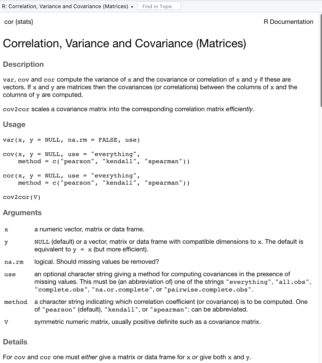
Help-file for the cor() function in R
In this help file you will see basic information about the function, what it does, which arguments it accepts, and what the output of the function is. Each help file follows the same structure, with the following parts.
- Description: A short description of the function, or family of functions are, what they are used for, and what they output
- Usage: A set of examples of how to use the function(s) and the default values of the arguments
- Arguments: A list of all arguments available for the function and what type of objects or values these arguments should take
- Details: A detailed description of what the function does, how it works, and how different arguments affect the behavior of the function. There may also be in depth discussions about the limitations of parts of the function, or special situations which may be of interest.
- Value: Details on what the output from the function are
- Note: Additional notes added by the authors of the function
- References: Books and/or articles that implementation of the function is built upon
- See Also: a list of related function with similar functionality that may be interesting for the reader
- Examples: One or more examples of how to use the function
If we look at the arguments section of the help file for the cor() function, you can see that there are six arguments listed there. However, not all of these can be used in the cor() function, since this help file is shared between several function. If you look in the ‘Usage’ section, you can see that only four of the six arguments are used in cor(), these are x, y, use, and method. However, when we used our function we did not specify the x and y arguments. Instead, we just input our two vectors as the first and second arguments and it worked regardless. Why?
Well, in reality, all arguments in R functions are named arguments. However, if you simply input the arguments in the correct order, R will interpret the first argument you have entered to be the first argument of the function, regardless of what that argument is named. Thus, when we input our two vectors, vote_share_per_district and voters_per_district, R assumed that these two vectors were corresponding to the first and second arguments, i.e. x and y of the function. When we added our method argument, on the other hand, we had to explicitly name this argument since method is the fourth rather than the third argument of the cor() function. See what happens if you now run the function cor(vote_share_per_district,voters_per_district, "spearman"), i.e. running the function without specifying that "spearman" is the method argument. You should get an error message which says:
> cor(vote_share_per_district,voters_per_district, "spearman")
Error in cor(vote_share_per_district, voters_per_district, "spearman") :
  invalid 'use' argument
As you can see, R interpreted "spearman" as the value for the third argument use instead of as the fourth argument method which is what we wanted. A good practice is therefore to always use named arguments in the function, unless you are absolutely certain of the order of the arguments.
4.3 Data types and classes
Thus far we have almost only worked with objects that are numbers. There are, however, a large number of different data and object types which you will encounter when learning R. You can check what the type of an object by running the function class() on the object.
> class(vote_share)
[1] "numeric"
As you can see, R tells us what we already know. That the object vote_share is a number, i.e. that it has the class "numeric".
There are a large number of different classes in R that you will encounter, but some of the most common ones are:
numericwhich are simply one numeric value, or a collection of numeric values known as a vectorcharacterwhich are made up of text and are usually referred to as strings. These strings are always enclosed by quotation marks. An object with classcharactermay also be a collection of strings, and is then known as a character vectorfactorwhich are a variable with multiple categories. These categories may be numeric or labelled (i.e. have names). In general, the classesfactorandcharacterare very similar, but behave differently in some cases. We will return to the differences between these two at a later stage.matrixwhich is a rectangular data structure with rows and columns. Matrices can be thought of as a collection of vectors where each vector corresponds to a single column or row. Importantly, matrices require that all the data inside the matrix are of the same type, for instancenumeric,character, orfactordata.frameortibblewhich are similar to a matrix, but allows for different data types inside the same data frame. Data frames are the general structure for data sets where each row corresponds to an individual observation, and each column corresponds to a variable. We will dive a bit deeper into the difference betweenmatrix,data.frameandtibblein the next chapter.
What class an object has affects what methods you can use on it and the default behavior of certain functions. For instance, correlations are only ever relevant between numeric values and trying to input a character vector in the cor() function will thus result in an error. This is evident from the Arguments section of the cor() help file where it clearly said that x and y had to be numeric arguments. Let’s say that we create a character vector of the names of the ten electoral districts in our example above, and try running a correlation between the district names and the vote shares
district_names <- c("Capital", "North", "North-East",
                    "North-West", "Western", "Central",
                    "Mountains-West", "Mountains-East",
                    "Big Island", "Small Island") # District names

# If you already created the vote_share_per_district object above you do not need to create it again
vote_share_per_district <- c(0.506, 0.583, 0.618,
                             0.445, 0.219, 0.461,
                             0.680, 0.280, 0.532, 0.612)
cor(district_names,vote_shares)
If you do this you will get an error message which says Error in cor(district_names, vote_shares) : 'x' must be numeric. I.e. since the object district_names is a character vector and not a numeric vector, we cannot run a correlation between these two vectors. Similarly, if you want to use mathematical operations such as + or - you cannot use objects which are not numbers. You can look up the class of any object by simply using the function class() on the object. Certain object will have multiple classes, and some will have only one. As we proceed through this companion book we will encounter more examples of how object classes affect the behavior of functions.
4.4 Packages
Now that we have a basic understanding of what objects, functions, arguments, and classes are we can turn to one of the most powerful strengths of R as a programming language: that anyone can write their own functions and make them available in packages. The open source nature of the R language allows user to define and write their own functions to do custom things in R. This is an incredibly powerful feature which may allow you to speed up your work a lot if you are mechanically doing the same thing many times, or allow you to build your own tools to answer the questions you are interested in. Writing your own functions in R is not at all complicated, and we will look at some simple examples of this in chapter 6. However, what makes the R community so vibrant is the possibility of writing your own functions and bundling them into a package which you can make publicly available to anyone. This means that if you have developed a tool which others may find useful you can allow to download and use your package to do these things. Similarly, by working in R you are able to utilize the over 17,000 unique packages which are available in R to do the most varied types of analysis.
A package in R is simply a collection of functions and/or data which the author has decided to make available, and which has passed some specific tests about form and function by the CRAN network. Once a package has been made available at CRAN, any R user can install the package by using the function install.packages("package_name") where you insert the name of the package inside the quotation marks. Once the package has been installed you can access the package by running the library("package_name") function. Sidenote: while you have to use quotation marks around the package name in the install.packages() function, the quotation marks around the package name are optional in the library() function.
We can try this out by installing the MLmetrics package which contains tools for evaluating model performance and then loading. Note that package names are case sensitive, so it is important to ensure you use capital letters at the appropriate places.
install.packages("MLmetrics")
library(MLmetrics)
You have now loaded the MLmetrics package and have access to all the functions available here. We can check this by for instance looking at the help file of one of these functions, for instance the RMSE function which calculates the root mean squared error of predictions compared to their corresponding true values. When you get to the help page for this function you can see at the top that it says RMSE{MLmetrics}, which indicates that the RMSE function is part of the MLmetrics package. This is also visible at the bottom of the help file where the package name and version is written out.
Packages are one of the main strengths of R, as the vast number of packages available means that you have access to a near infinite pool of tools that have been developed by user all around the world and by users in all types of fields. Whenever you find yourself lacking a specific tool to do a specific thing in R, chances are that someone else have already developed a tool for doing it and have made it available through a package. To find the appropriate packages to use, the most useful way is simply too search online ‘how to do X in R’ and you will most likely end up finding a package which allows you to do X in R.