7 Data please!

7.1 Why do we use data?
Just like Johnny-five and his cousin the Robot cash register, Economists need ‘input’ from the real world to improve our understanding.
Descriptive
To measure and understand our object of study: the economy (including individuals, households, firms, and governments)
Levels of variables, patterns (e.g., Life cycle consumption),
observed relationships between variables (differences by group, correlations, linear relationships, etc.)
For its own sake
To use in executing policy (e.g., the Consumer Price Index)
To generate hypotheses and “calibrate” our models
We can have statistical tests of “descriptive” hypothesis.
E.g., testing
H0: Incomes of men and women are the same ceteris paribus vs. HA: Women with the same characteristics as men earn less on average.
Note: this is not testing a causal relationship;
a difference doesn’t necessarily imply a particular explanation (e.g., sex discrimination).
Causal: To make statistical inferences (and statistical predictions) about effects
(sometimes called “causal effects” but I find that redundant).
To measure and test hypotheses about the causal relationship between important factors and outcomes.
7.2 What data do you need to answer your question?
Look for data that is…
Relevant to your topic
the relevant population, years, fields;
relevant outcome variable(s), “independent variable(s)” of interest, control variables)
Useful for answering your question
e.g., contains a useful “instrumental variable”, a long enough time series, or repeated observations on individuals to allow ‘fixed effects’ controls
Reliable, accessible, understandable
Consider: What data have previous authors used to answer this or related questions?
7.3 Some types of data
Survey and collected data: self-reports, interviewers, physical measures and visual checks
Administrative data (e.g., tax records)
Transactions/interactions
- Scanner data
- Web data (e.g., Ebay, Amazon)
- Price data
Public financial data and company reports
Official government data (public releases and announcements, e.g., budget data)
Data from lab experiments
Data from field experiments
Consider the differences between:
Micro-data (individual/transaction level) vs. Macro-data (aggregated to firm, region, country-year level etc)
Panel vs cross-section vs time-series data
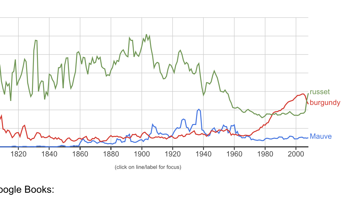
Figure 7.1: A graph based on a new type of data
Some examples of datasets used by Undergraduate students
Workplace Employee Relations Survey: Private Sector Panel, 1998-2004 data, from the UK Data Archive.
Data on cigarette consumption from the US Centers of Disease Control (CDC) from 1986 to 2011, for 50 states \(\rightarrow\) 1300 observations.
The 1958 National Child Development Survey, a longitudinal study tracking a group of individuals born in a single week in 1958.
Data on UK cities’ population, employment, geography, extracted from various ONS tables.
“The ICCSR UK Environmental & Financial Dataset, is a large panel data set on a a sample of firms, giving a set of ratings on “community and environmental responsibility”; merged to a set of financial variables on these firms, collected from Datastream
Exchange rates between the US dollar, the British pound, Australian dollar, Canadian dollar and Swiss franc, for the period 1975-2010, from the OECD Main Economic Indicators database.
The World Bank Development Indicator database (2013); 210 countries over a 20-year period from 1991-2010
65 banks over 8 years from BankScope (profitability measures, etc)
7.4 Getting and using data
Finding data
Update: A particularly promising resource: Google dataset search
In searching for data, note that the American Economics Association has a very comprehensive list of links: http://www.aeaweb.org/RFE/toc.php?show=complete for the UK in specific, see http://www.statistics.gov.uk/default.asp
For macro and micro data, see http://www.esds.ac.uk/
For large scale data, see also the UK Data Service database.
Some other sources of data, and links to aggregations on my webpage here.
Some of these (and lists of lists) are also listed in this Airtable also mentioned below… this is filtered ‘data search/archive’; remove this filter to see more.
Also, to comment on this you can get full ‘commenter’ access link
Also note that data from published papers are typically expected to be made publicly accessible (for replication and checking purposes). If you cannot find it on the journal or the author’s website (or linked therein), you can email the corresponding author to ask for it.
Don’t wait too long to begin collecting your data and producing simple graphs and summary statistics, to get a sense of your data.
Empirical work is difficult and you may not be able to get the “best” data This is OK. Remember, at the undergraduate/MSc level, we generally want you to show your competencies in these assignments; we expect the analysis will have limitations.
7.4.1 Downloading the data, raw formats
The most common format to download the data in is ‘csv’ for ‘comma-separated values.’ This can be read into Stata, R, and nearly any program.
The first row usually gives the variable names, which you can change later in your program.
Commas separate each variable (aka ‘feature’ aka ‘column’).
Each observation (aka ‘unit’ aka ‘row’) is separated by a line break.
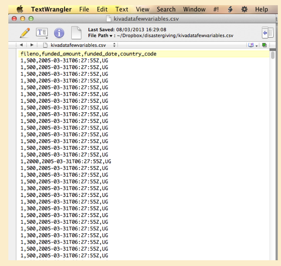
Figure 7.2: Raw data viewed in a text editor
(See ‘Text editors’ below.)
7.4.2 Inputting the data (into Stata, R, etc)
These programs have several ‘input’ commands you can use (e.g., insheet in Stata, read_csv in R) for “getting the data in” (as an object that can be referred to and analyzed).
7.5 Understanding your data
Present simple statistics and graphics on your data before doing more involved analyses.
7.6 What does data look like (brief)
Author’s note to self: Display these directly through R, especially using the built-in datasets
Observations, variables
Each “unit” is an observation. Think of these as the rows of a spreadsheet.Every unit will have values for each of the “variables”. You may create new variables from transformations and combinations of the variables.You may limit your analysis to a subset of the observations for justifiable reasons. Your analysis may need to drop some observations, e.g., with missing variables (but be careful).
7.6.1 Cross-sectional, time-series, and panel data
An example of…
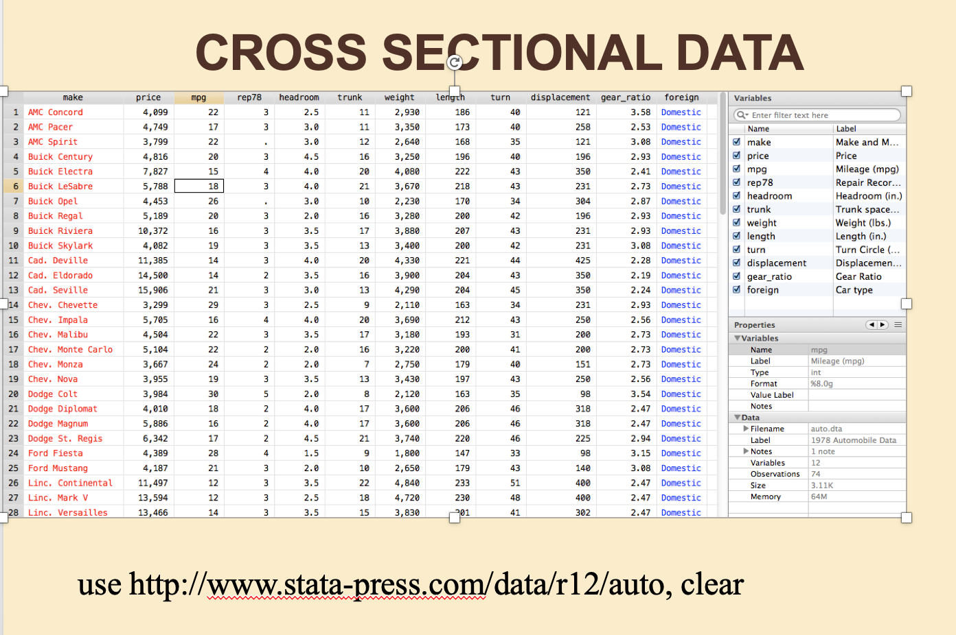
Figure 7.3: Cross-sectional data
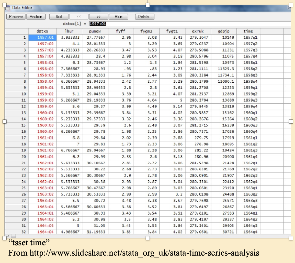
Figure 7.4: Time-series data
Time series: A single ‘unit’ over time… in this case 4 quarters per year, shown in Stata’s ‘data editor’. (But you shouldn’t usually edit data in this mode – do it with code!)
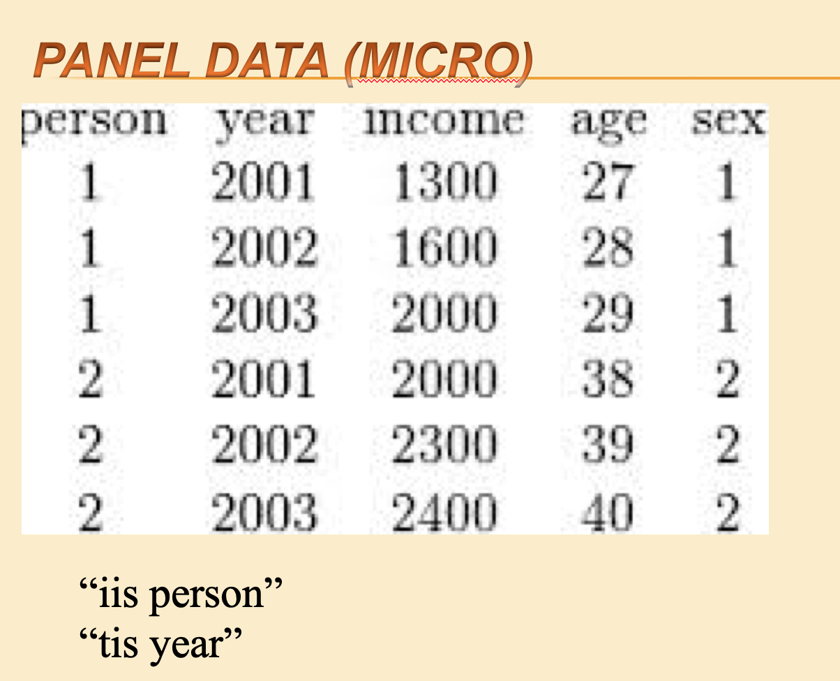
Figure 7.5: Panel data (micro)
xtset is a Stata command to tell Stata you are dealing with panel data. Within this command you specify the variable identifying the unit with iis and the variable identifying the time period with tis.
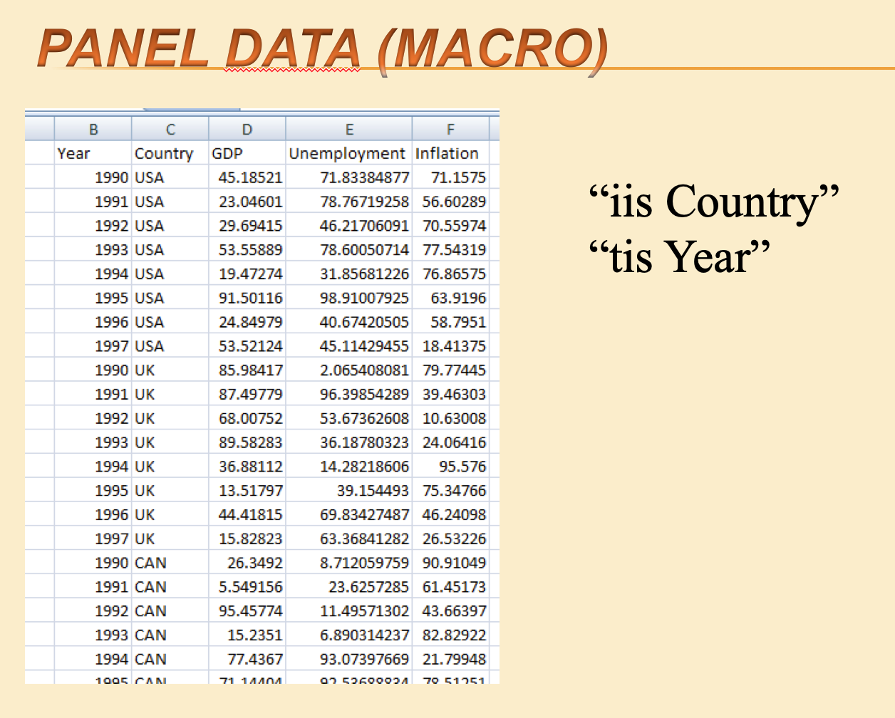
Figure 7.6: Panel data (macro)
Above: Cross-country panel data
String and numeric variables
String variables are text. In their raw form, they usually have quotes (“john smith”,) around them.
Numeric variables can be integers, “floats”, etc, stored in various forms. They are numbers.
Most statistical packages and programming languages treats these two types of variables differently, with a different “syntax” and different commands for each. Be careful.
There are many other data types, with some variation in how these are categorised and stored between languages. E.g.,
‘Factor’ variables (categorical, ordinal)
Logical (true/false)
Date and time variables
7.7 Doing ‘coding’: cleaning, visualizing/summarizing, analysing, and presenting
Some quick important guidelines
Do ALL of your work (cleaning, merging, creating variables, and analysis) by writing code in a ‘script file’ (Stata – a ‘.do file’; R – a ‘.R’ or ‘.Rmd’ file; Python– a ‘.py’ file, I think)
Do your cleaning/construction and analysis in separate files (or at least separate parts of the same file; clean the data first, then analyse it)
Keep this organised, and try to write it in a way that you, or others, could return to it later.
A good reference… but getting old now: (“Code and Data for the Social Sciences”, 2014, Gentzkow and Shapiro)[https://web.stanford.edu/~gentzkow/research/CodeAndData.pdf]
Some other resources (more up-to-date?) listed Here
7.8 Doing an econometric analysis
Which techniques
You may not be able to use the “ideal” estimation technique; it may be too advanced. But try to be aware (and able to explain) of the strengths and weaknesses of your econometric approach.
Time series, cross section, or panel data?
“A major problem is always understanding the difference between a panel and a time series. My students always want to just do a time series regression, and don’t understand why the cross-section dimension is important.” –University of Essex lecturer
Common difficulties
Diagnostic tests, etc.
Interpreting your results
“The second most frequent issue is that they think they are supposed to get a ‘right’ answer. They stress out when the regression doesn’t come out ‘right’.” – University of Essex lecturer
7.9 Presenting your results
Considering alternative hypotheses and “robustness checks”
Of course it’s OK to use these menu items at first, and to help you find the command you are looking for. When you use the drop-down menu you should also be able see which code it enters into the command window/console, and use that in your own script.↩