Chapter 4 Workshop 3: Genome browsing
4.1 Browsing the human genome
In previous practicals, you have downloaded small microbial genomes onto your local computer and browsed them using the IGV software. We can, in principal, do the same thing with the human genome. However, it is usually more convenient to use one of the freely available web-based human genome browsers. The most popular human genome browswers on the web include:
Both of these browsers are rich with large amounts of data overlaid onto a human reference genome sequence. Let’s use these to try to solve Weblem 9.1 from Lesk’s Introduction to Genomics.
4.1.1 What gene appears between the genes for C4A and C4B in the human genome?
Both of these browsers are rich with large amounts of data overlaid onto a human reference genome sequence.
Let’s use these to try to solve Weblem 8.1 from Lesk’s Introduction to Genomics.
In Ensembl (https://www.ensembl.org/Homo_sapiens/Info/Index), let’s try searching for ‘C4A’:
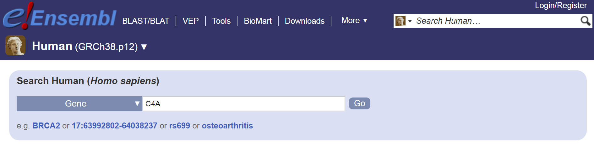
Search form
4.2 Handling “next-generation” sequencing (NGS) data: alignments against a reference genome
NGS data from shotgun sequencing of a genome typically generates very large numbers of short sequence reads. Today, we are going to see how we can make some sense of the data, by viewing the reads aligned against a reference genome sequence.
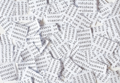
Making sense of short sequence reads is something like piecing together text on scraps of paper from a shredder. There are two main approaches:
- alignment against a reference genome sequence and
- de novo assembly.
Here we will look at the former (alignment).
4.2.1 The data
The sequence data that we are using today comes from the genome (and transcriptome) of the bacterium Mycobacterium tuberculosis, a bacterial pathogen that infects about 2 billion people (a third of the world’s population) and is the causative agent of tuberculosis.
Its genome is small and therefore convenient to work with. The same principles that we learn about today are mostly applicable for larger genomes too but would require more time and computer resource to analyse. Specifically, we will be using genomic sequence data from a survey of tuberculosis transmission in Oxfordshire (Campbell et al. 2018) and a transcriptomic dataset from another as-yet unpublished study.
Both these datasets consist of pairs of short reads, generated using Illumina sequencing. We will also take a look at a genomic sequence dataset generated using PacBio (Pacific Biosciences) longer reads (Philip et al. 2016).
As the reference genome sequence, we will use the completely assembled sequence of strain H37Rv (Cole et al. 1998). In advance, I generated some alignment files for you; the sequence reads were aligned against H37Rv reference genome sequence using a software package called BWA.
| SRA accession number | Genome / transcriptome | Strain of M. tuberculosis | Sequencing method |
|---|---|---|---|
| ERR400344 | Genome | OxTb-6 | Illumina HiSeq |
| ERR400311 | Genome | OxTb-321 | Illumina HiSeq |
| SRR3667790 | Genome | SB24 | PacBio SMRT |
| SRR5061507 | Transcriptome | H37Rv | Illumina HiSeq |
| SRR5061515 | Transcriptome | H37Rv | Illumina HiSeq |
All of the files that you need are available via the “Workshop 3. Link to example data” item on the University of Bristol Blackboard page.
4.2.2 The software: IGV
To interactively browse the genome, and the NGS sequence data aligned against the genome, we are going to us the Integrative Genomics Viewer (IGV) (Thorvaldsdottir, Robinson, and Mesirov 2013). You may need to either download and install the IGV software or you can use the web-based version, which requires no installation; you just access it through your web browser. Under some circumstances this version runs much more smoothly than the locally installed version. The disadvantage is that some of the details of the menus and functions etc. are slightly different than those in the locally installed version; so, you may need to ask for help if you get stuck with this.
I have recorded a video to show how to use the IGV web application here.
I also recorded a video showing IGV in action here. I use a Mac, but it is not very different on a Windows-based PC.
4.2.2.1 If you want to find out more:
- An online tutorial for the locally installed IGV is available from here.
- A tutorial video is available here: https://www.youtube.com/watch?v=YpNg0hNUuo8, which uses some human genome data.
- For the web-based version of IGV, help is available at this site, here.
However, by using this document and a bit of trial and error you should be able to quickly learn how to use IGV without needing to access those tutorial materials.
4.2.3 What you need to do
First, download the data from the OneDrive (see link above).Then, you need to follow the steps described below. These will lead you through how to load the reference genome the aligned NGS reads into IGV. You then need to play around with IGV and learn to drive it. Try to answer the questions below.
4.2.4 Loading the reference genome into IGV
When you first start (the locally installed version of) IGV, it will look something like this:
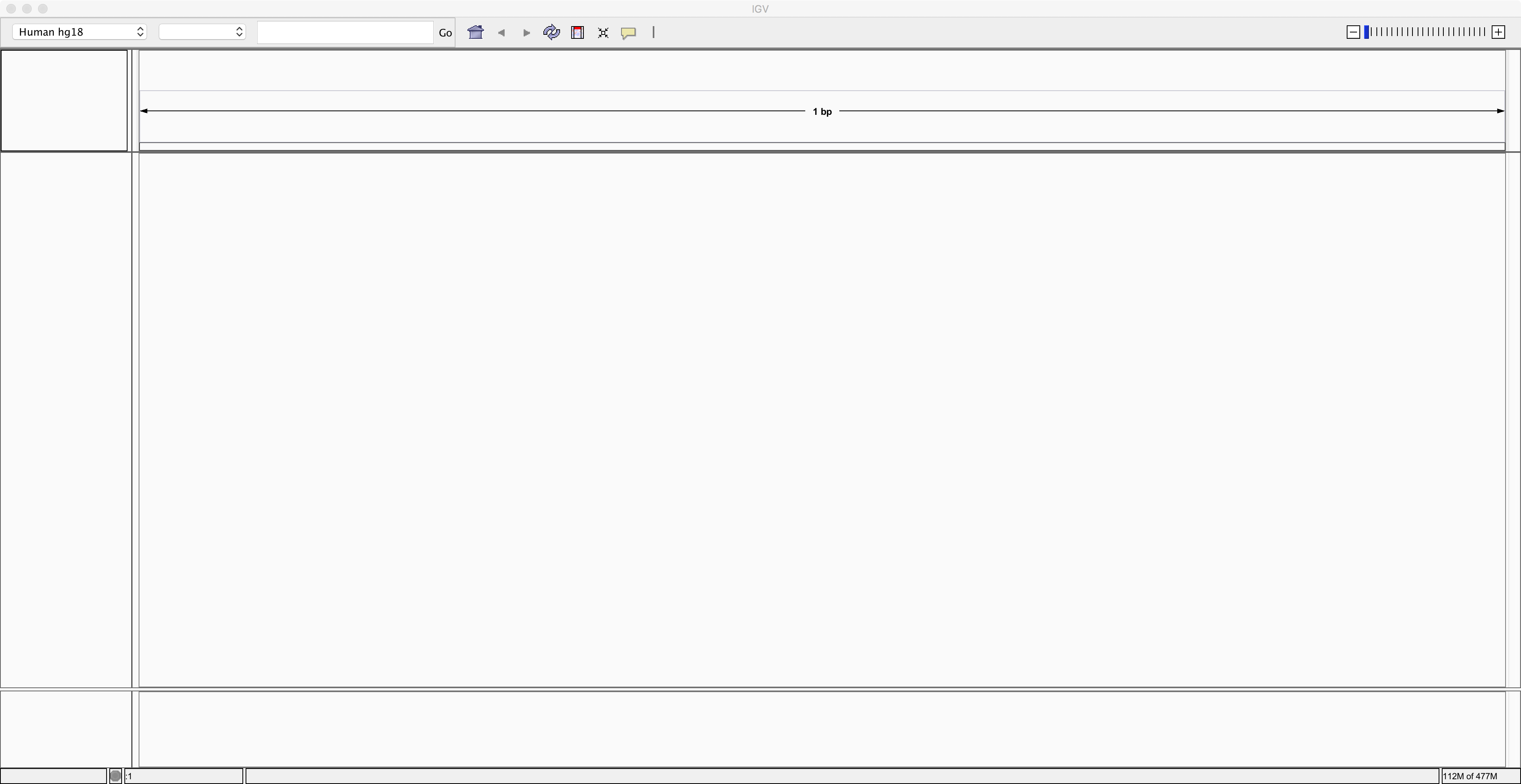
If you are using the web-based version of IGV, it looks sightly different. See the section called “Using the web-based version of IGV” later in this document.
To load the nucleotide sequence of the reference genome, locate the
“Genomes” menu item. Choose “Genomes -> Load genome from file” and
locate the reference genome sequence file that you downloaded earlier.
This file should be called GCA_000195955.2_ASM19595v2_genomic.fna.
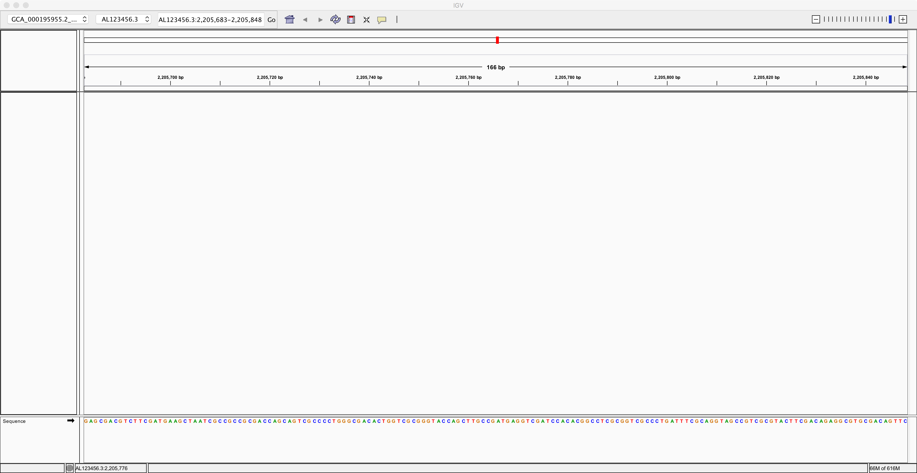
Once you have loaded this reference genome sequence, use the control near the top right corner of the IGV window to zoom in as much as you can. Then you should be able to see the nucleotide sequence of the reference genome along the bottom:
Next, we need to load the genome annotation. Use the menu item called
“File -> Load from file” to select the annotation file that you
downloaded earlier. This should be called
GCA_000195955.2_ASM19595v2_genomic.gff. After loading the
annotation and zooming out a bit, you should see something like this:
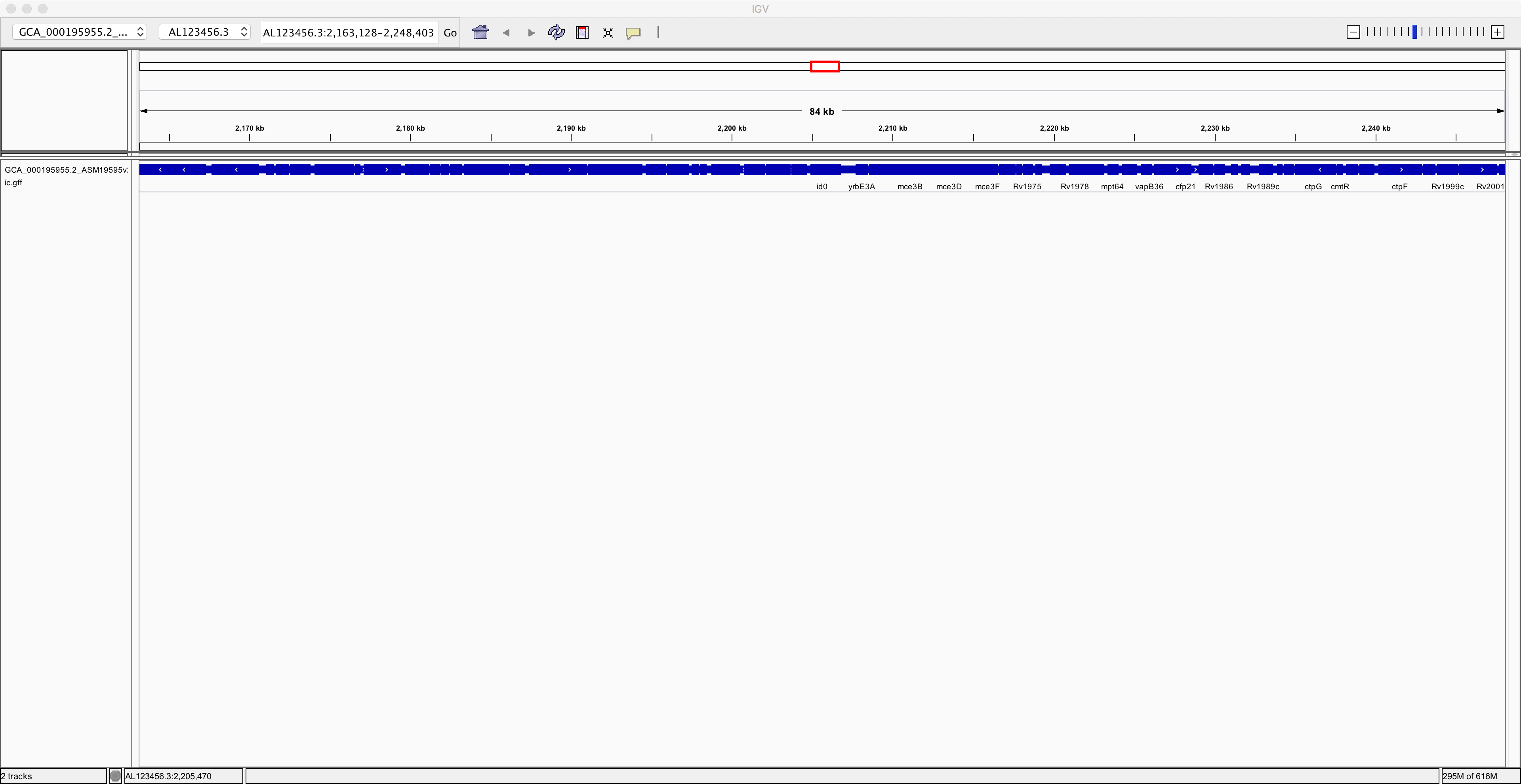
Notice that you have now added an extra track containing the annotation of the genome. Next, to improve clarity, right-click on the annotation track and select the “Expanded” option. Now you can see the individual genes more clearly on the reference genome:
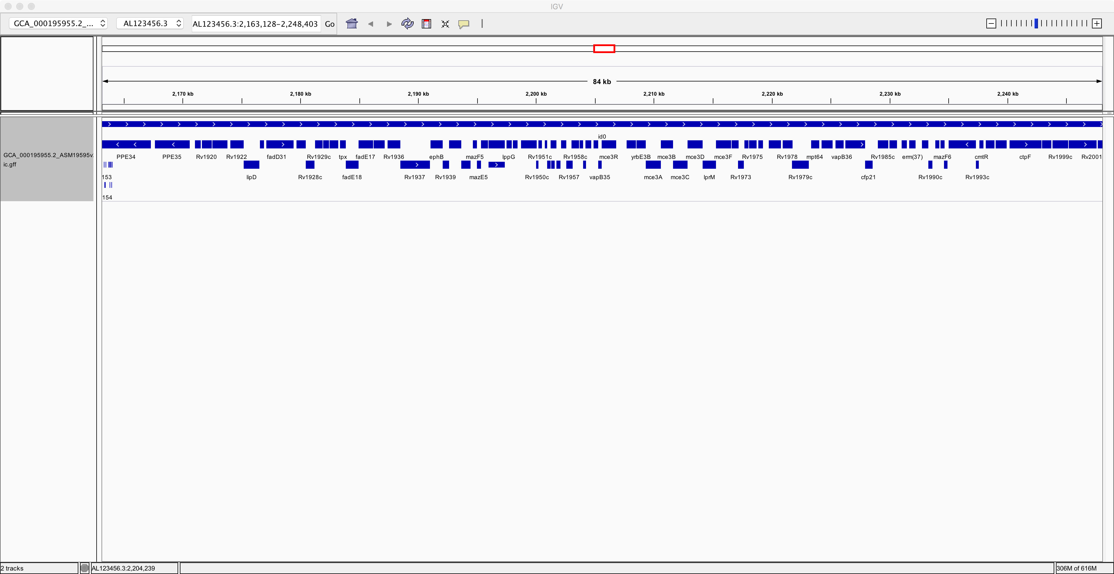
Now spend at least a few minutes learning how to navigate around the genome, zooming in on specific regions and finding information about specific genes:
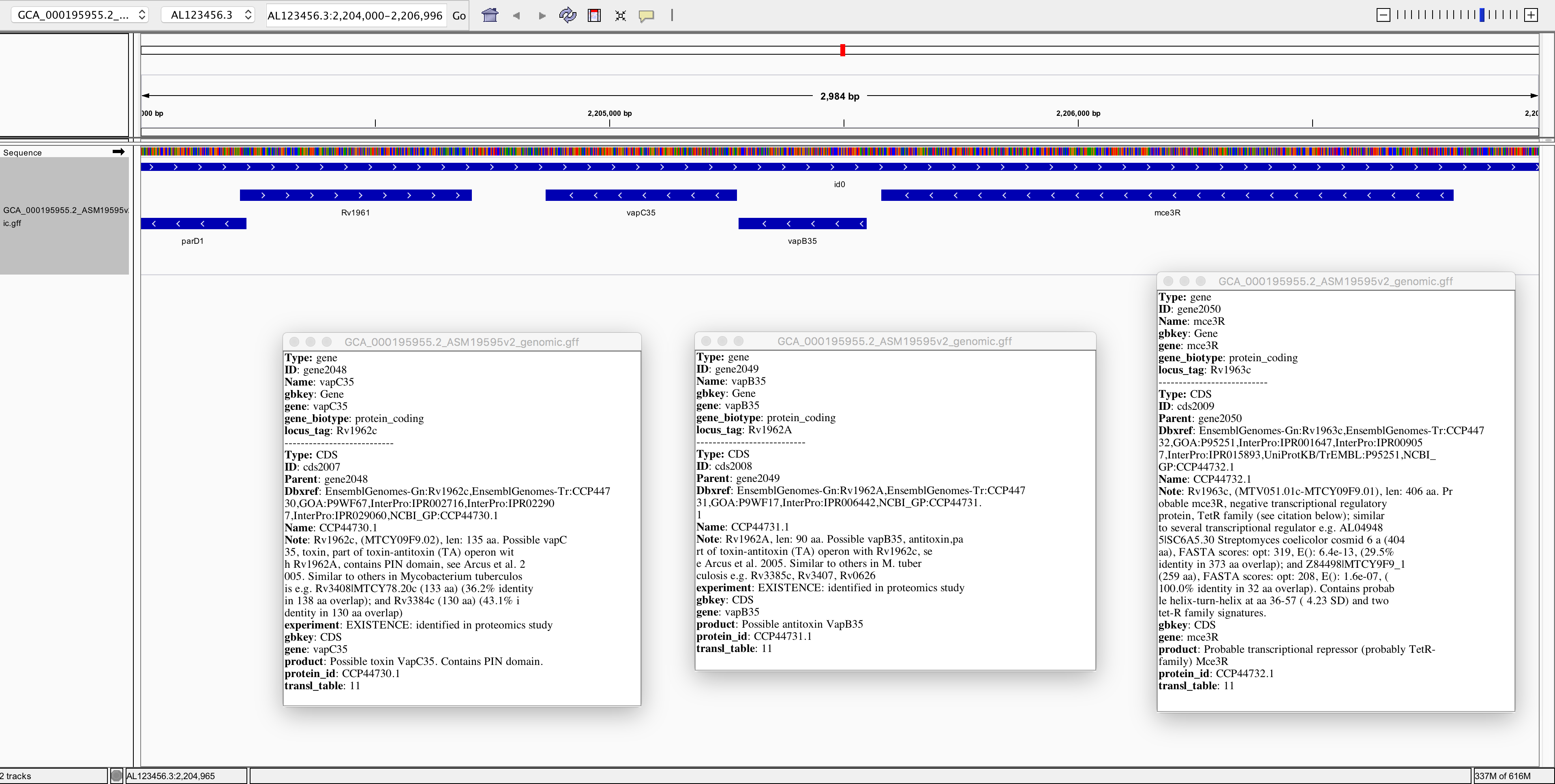
Note that you can navigate to specific sites on the genome or search for specific genes, using the search field near the top:
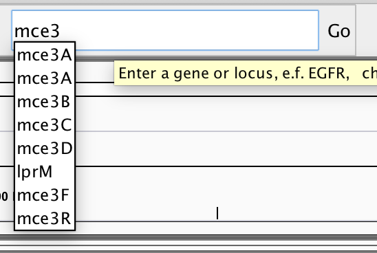
You might wish to locate genes of particular interest that are involved in virulence of this pathogen, e.g. katG, hspX (acr), erp, hma, pcaA. Once you are confident that you understand what you are looking at and are reasonably adept at navigating around the genome, then please proceed to loading the alignment data into IGV.
4.2.5 Loading the alignments into IGV
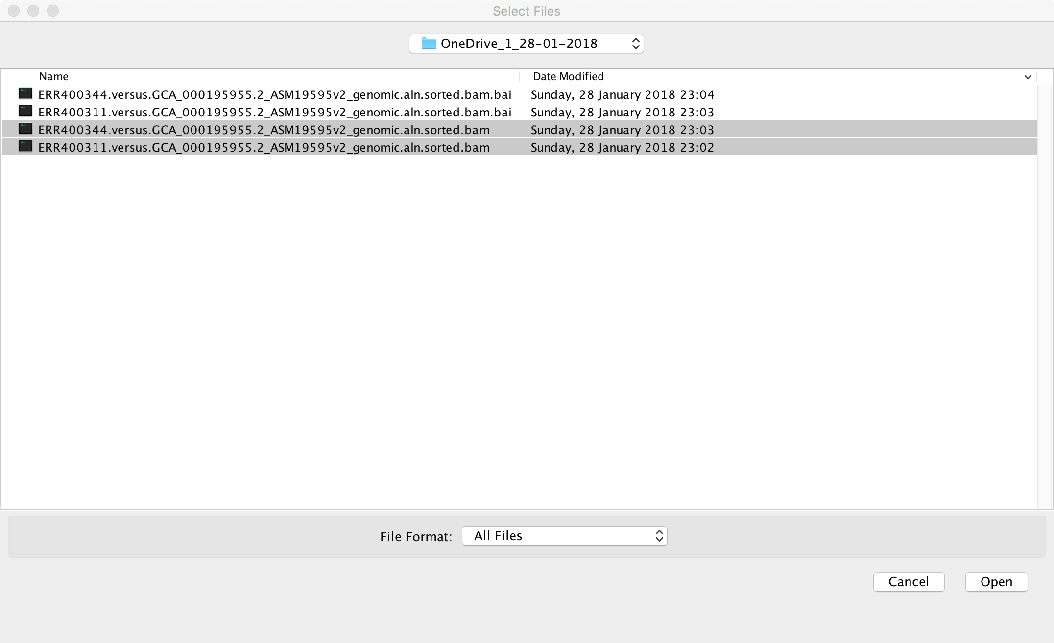
Use the “File -> Load from file” menu item to load the alignment
files that you downloaded earlier. The names of these files should end
in .bam. Please note that you also need to have the index files
(.bam.bai) present in the same folder. In the screenshot below, I am
loading two alignment files:
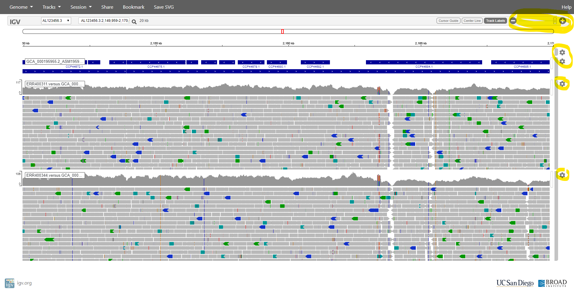
After loading these two alignments of genomic reads, we see something like the following screenshot. Please note that right-clicking on various parts of the window brings up menus that allow you to configure and rename tracks.
What is this ‘alignment data’ that you have added (from the .bam files)? It is the result of aligning each sequence read against this reference genome sequence. Make sure that you understand the following concepts:
- DNA sequencing
- Shotgun DNA sequencing
- A sequence read
- Sequence alignment
- Aligning sequence reads against a reference genome sequence
- Coverage depth
- “Paired-end” DNA sequencing
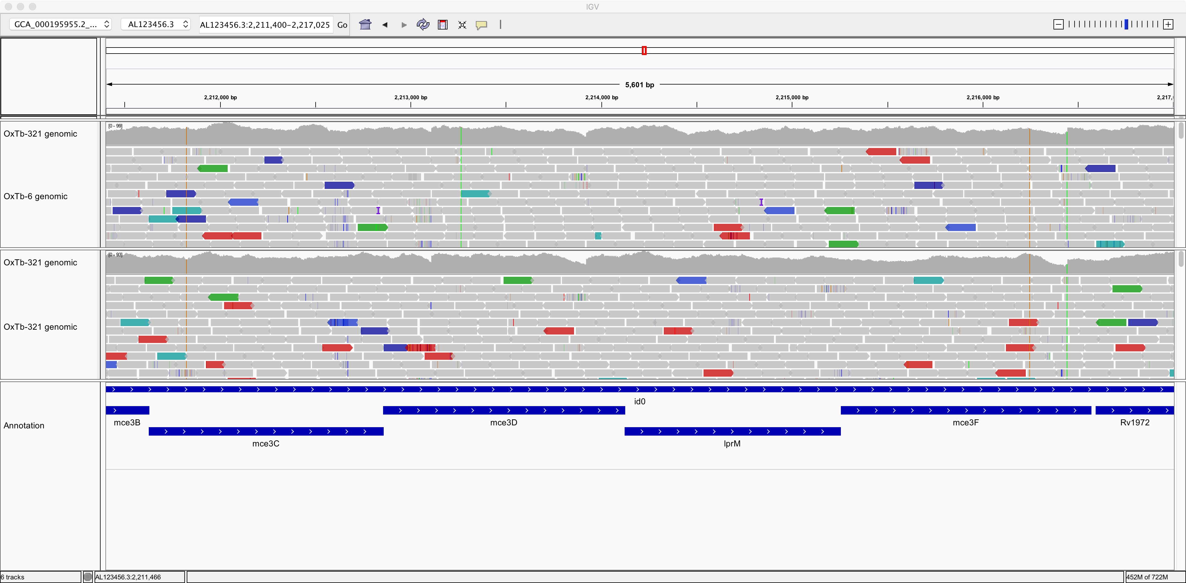
So, now we can see individual sequence reads aligned against the reference genome. We can also see plots of coverage depth.
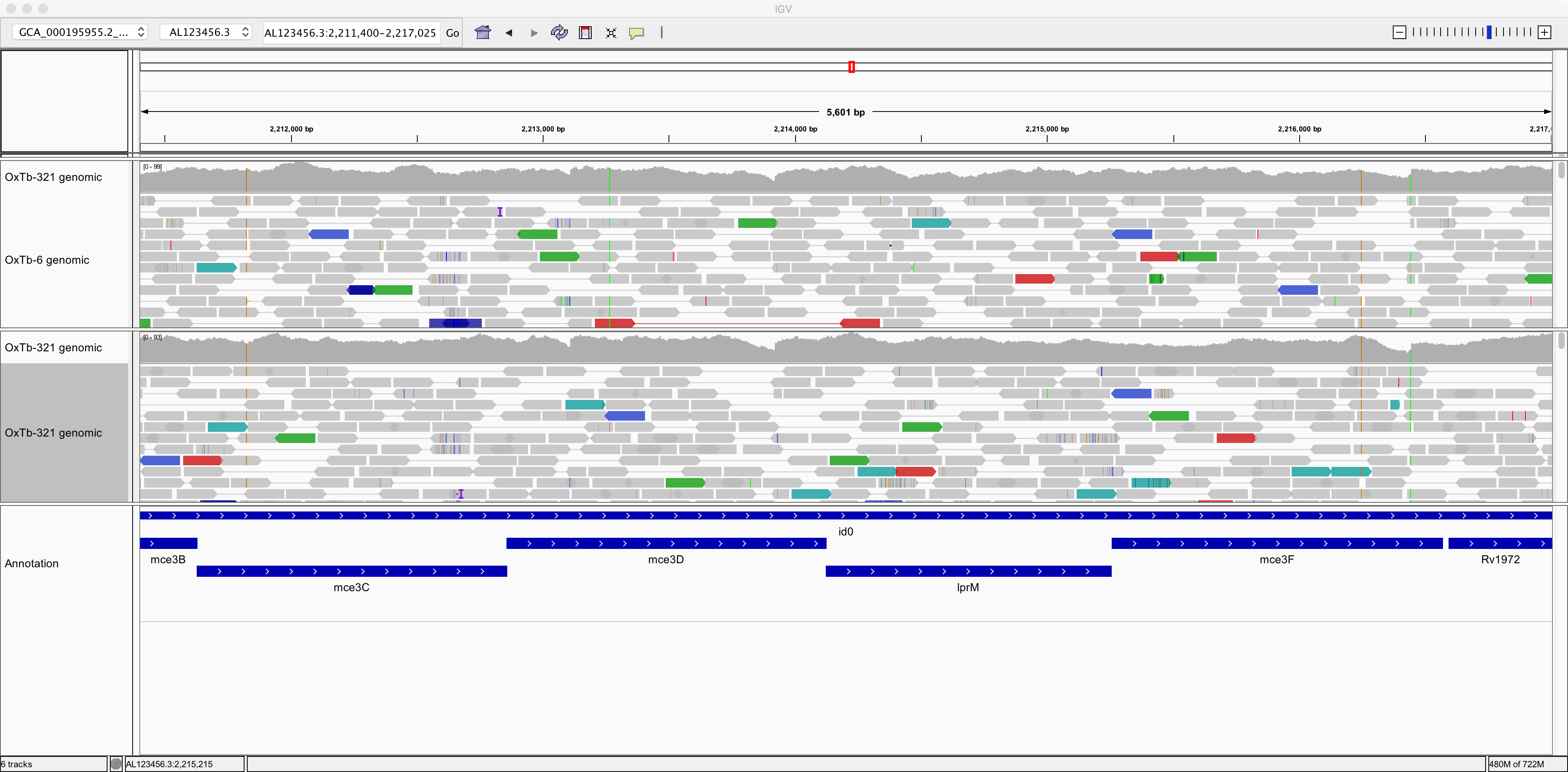
Now let’s right-click on the tracks and choose the option to “View as pairs.” Now we can see pairs of reads joined by a thin horizontal line. This pairing arises from the fact that sequencing was performed at both ends of the genomic fragments.
| Question | Answer |
|---|---|
| What size, approximately, were the fragments of genomic DNA in these two samples? | |
| What do you think is denoted by the different colours of the sequence reads? |
Now let’s zoom in on position AL123456.3:2,213,265:
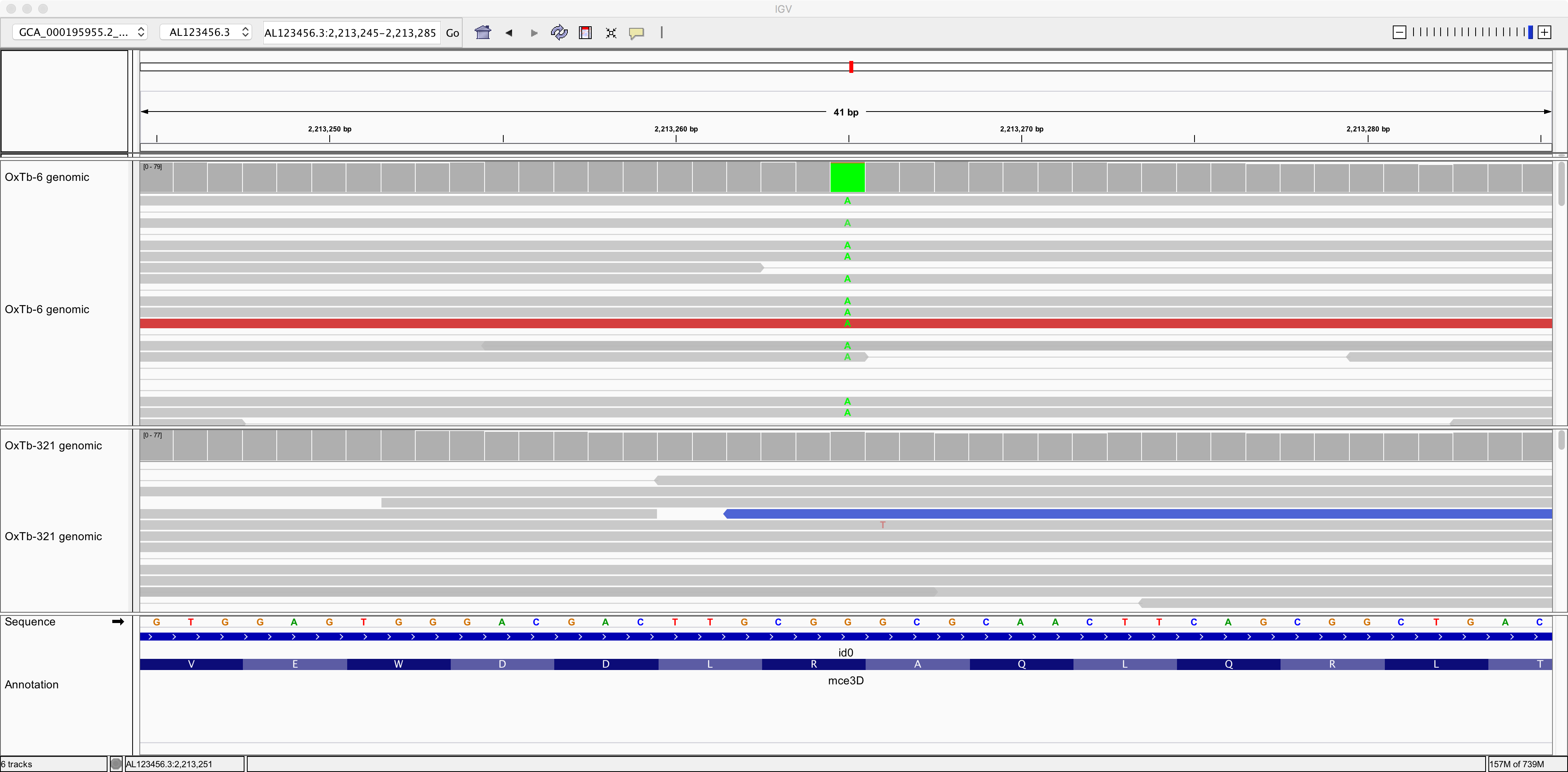
Here we can see a single-nucleotide polymorphism (SNP). Both the reference genome and strain OxTb-321 have a G at this position; but strain OxTb-6 has an A.
Do you think this G/A SNP will have any impact on an encoded protein? Why?
Now, try to find a few more SNPs:
| Genomic position | Reference base | Alternative base | Effect on protein |
|---|---|---|---|
Now, take a look at this genomic region: AL123456.3:2,232,639-2,244,376.
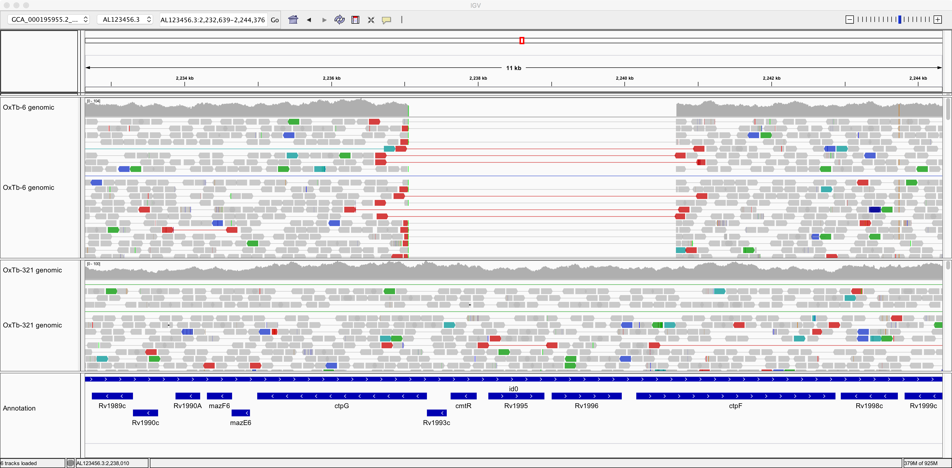
Here, strain OxTb-6 appears to lack a genomic region comprising 4 genes that are present in the reference and in OxTb-321. Notice how the read pairs span across the gap in OxTb-6. Can you find any other genes missing from OxTb-6 and/or OxTb-321?
Now let’s take a look at the genomic data generated using the PacBio method. This is in file
SRR3667790.versus.GCA_000195955.2_ASM19595v2_genomic.aln.sorted.bam.
Notice how the reads are much longer but contain numerous errors:
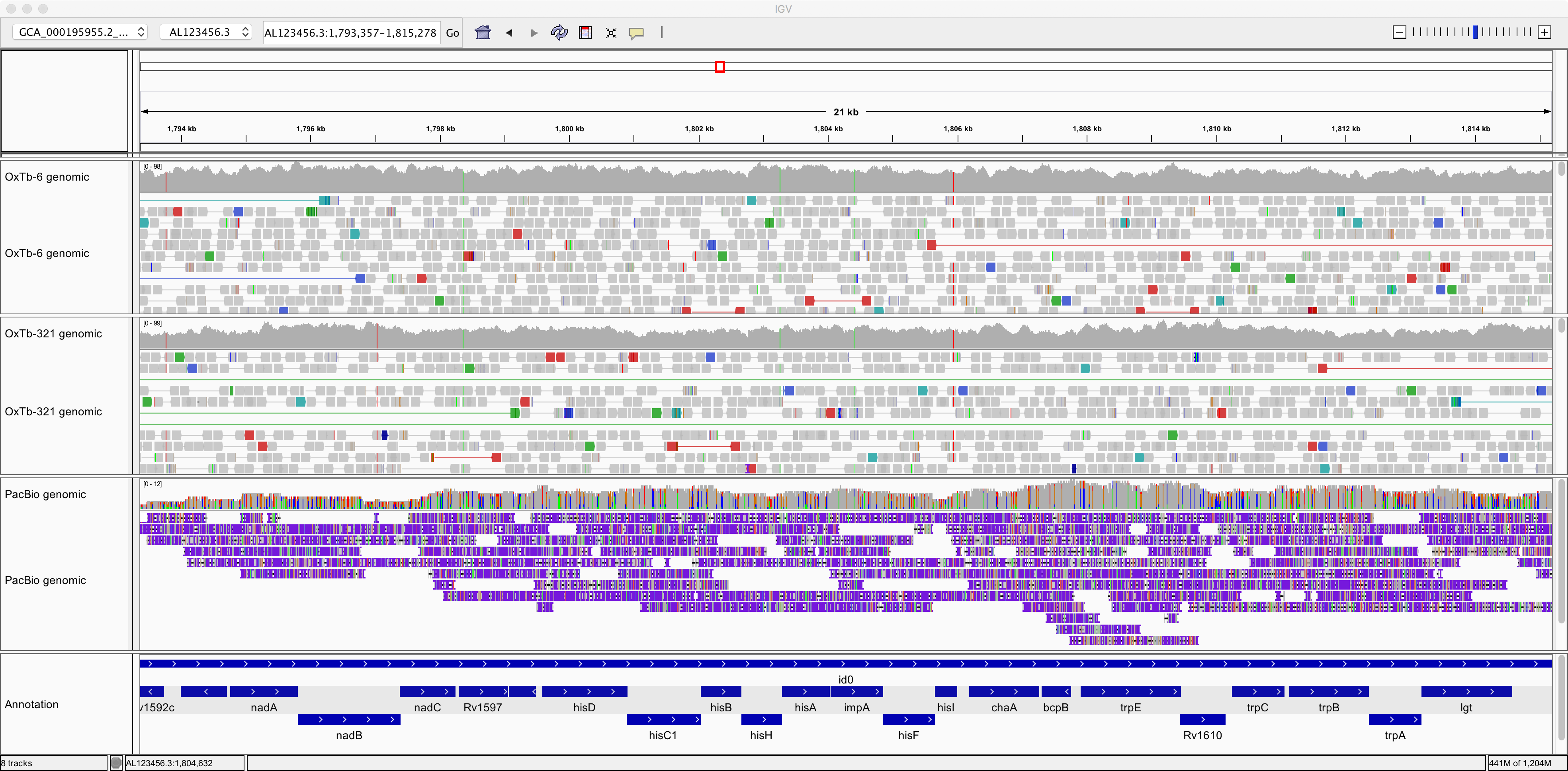
This illustrates the trade-off between read-length and read-accuracy that we are faced with when deciding the best strategy for sequencing a genome. In practice, often researchers have used a combination of Illumina plus PacBio sequencing, using short, accurate Illumina reads to correct the errors in the long, innaccurate reads. (More recently, the accuracy of PacBio sequencing has improved dramatically, such that it is now feasible to use only long PacBio reads; but the databases still contain a lot of poor-quality legacy data).
Now, let’s take a look at some transcriptomic data. Use “File -> Load
from file” to load alignment files
SRR5061507.versus.GCA_000195955.2_ASM19595v2_genomic.aln.sorted.bam
and SRR5061515.versus.GCA_000195955.2_ASM19595v2_genomic.aln.sorted.bam.
This data consists of Illumina sequencing of fragments of cDNA (i.e. DNA generated in the lab by reverse-transcribing messenger RNA). It therefore presents a survey of the sequences mRNA transcripts present in the cell. The two samples were prepared from the same bacterial strain but under different growth conditions.
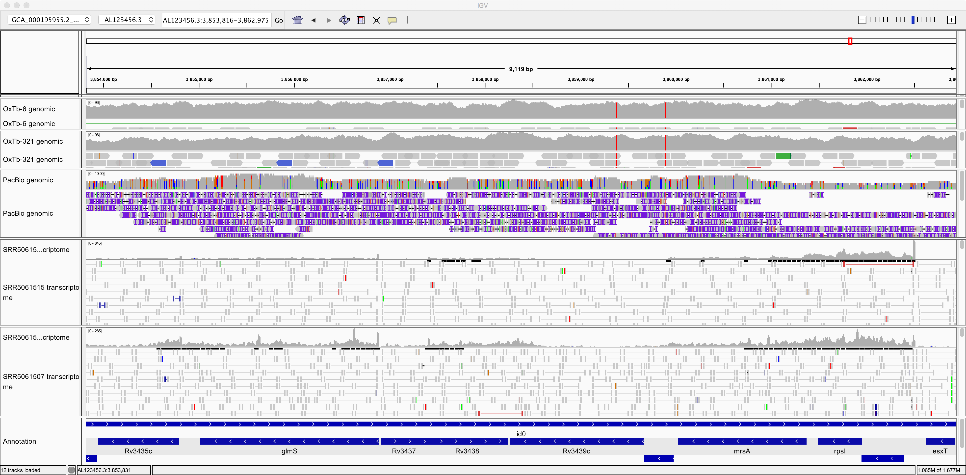
Note that the transcriptomics data looks quite different from the genomic data in a few respects. Make sure you understand the reason for each of these:
The depth of coverage by genomic sequence is more uniform than by transcriptomic sequence.
There are many “gaps” on the reference genome with little or no coverage by transcriptomic sequence.
There tend to be fewer mismatches between the RNA-seq sequences and the reference genome than is the case for these genomic datasets.
Also note in the image above, it seems that gene glmS is significantly more expressed (transcribed) in one sample than in the other. Can you find any more examples of such differentially expressed genes (DGEs)?
4.2.6 Qualimap: QC and summary statistics for alignments
Qualimap is a program that generates summary statistics for an alignment of reads against a reference sequence. It’s primarily a technical tool which allows you to assess the sequencing for any problems and biases in the sequencing and the alignment rather than a tool to deduce biological features. There is a lot of information in the report so here are just a few highlights:
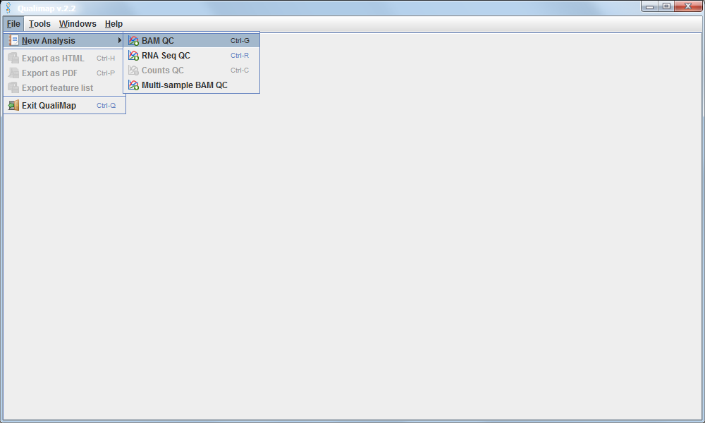
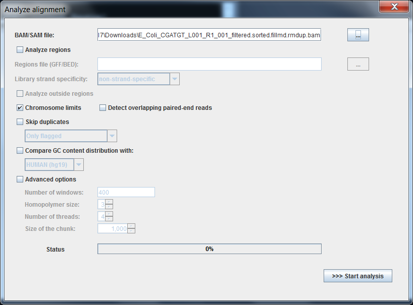
4.2.7 Loading a BAM file into Qualimap software:
Recall that the alignment data is contained in the .bam file. So we must load this file into the Qualimap software.
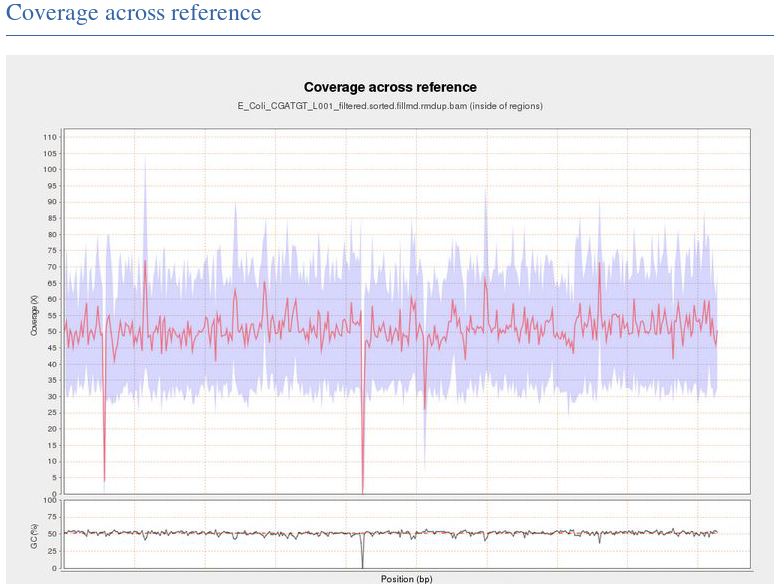
This shows the number of reads that ‘cover’ each section of the genome. The red line shows a rolling average around 50x - this means that on average every part of the genome was sequenced 50 times. It is important to have sufficient depth of coverage in order to be confident that any features you find in your data are real and not a result of noise (sequencing errors).
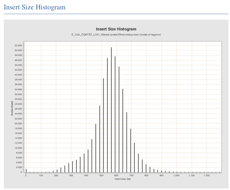
The Insert Size Histogram displays the range of sizes of the DNA fragments that were sequenced. Note that the ‘insert’ refers to the DNA that was inserted between the sequencing adaptors, so equates to the size range of the DNA that was used. Recall that paired-end sequencing involves sequencing both ends of each fragment. Therefore, after aligning both ends against the reference, it is possible to measure the distance between each end of the fragment with respect to their positions in the reference genome.
In this case we have paired 300-base reads and our insert size is around 600 bases; so there should only be a small unsequenced gap between the pair of reads.
Have a look at some of the other graphs produced with your alignment files and try to figure out their meaning and significance.
4.2.8 What next? Comparative genomics of Cyberlindnera fabianii
You have now covered the essential material. If you still have time and want some further challenge, then optionally let’s work through an example using the yeast Cyberlindnera fabianii.
You will see from the published literature that this yeast can cause fungaemia in human patients, albeit rarely.
Now, you should apply the skills you have learned in these practical,excercise to the C. fabianii data to find some interesting features of its genome and/or differences between different strains. All of the files that you need are available via the links on the ELE page, here.
Below we work through an example.
By searching the NCBI Entrez web portal, you can see that there are several genome assemblies available for this species:
| Strain name | Assembly accession number | SRA accession number |
|---|---|---|
| YJS4271 | GCA_003205855.1 | n/a |
| 65 | GCA_001983305.1 | SRR5047278 |
| JCM 3601 | GCA_001599195.1 | DRR032607 and DRR032482 |
| Ex2 | GCA_004195225.1 | n/a |
Can you find out any information about these genome sequencing projects? For example, are there any published papers describing these genome? try to fill the missing information in this table:
| Strain | Source | Genome annotated? | Published paper |
|---|---|---|---|
| YJS4271 | Yes | ||
| 65 | |||
| JCM 3601 | Shen et al. (2018) Tempo and Mode of Genome Evolution in the Budding Yeast Subphylum. Cell. 175:1533-1545.e20. | ||
| Ex2 | Clinical sample, Exeter | No | None |
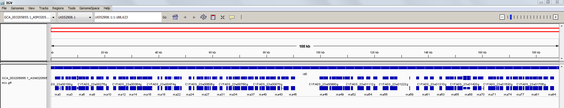
Let’s load the genome of C. fabianii YJS4271 into the IGV viewer. First we load the genome sequence file
GCA_003205855.1_ASM320585v1_genomic.fna (using the ‘Genome’ menu) and then the annotation file GCA_003205855.1_ASM320585v1_genomic.gff (using the ‘File’ menu). Expand the annotation view, zoom into a
specific place in the genome and it should look something like this:
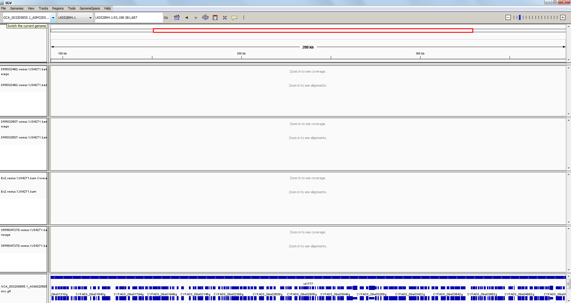
Now, let’s load the files containing alignments of sequence reads against the YJS4271 reference genome sequence.
Using the ‘File’ menu, we will load the following files:
DRR032482.versus.YJS4271.bam,
DRR032607.versus.YJS4271.bam,
Ex2.versus.YJS4271.bam,
SRR5047278.versus.YJS4271.bam
Remember that for each .bam file you need to have the corresponding .bam.bai file also in the same directory.
After loading the .bam files, your IGV should now look something like this:
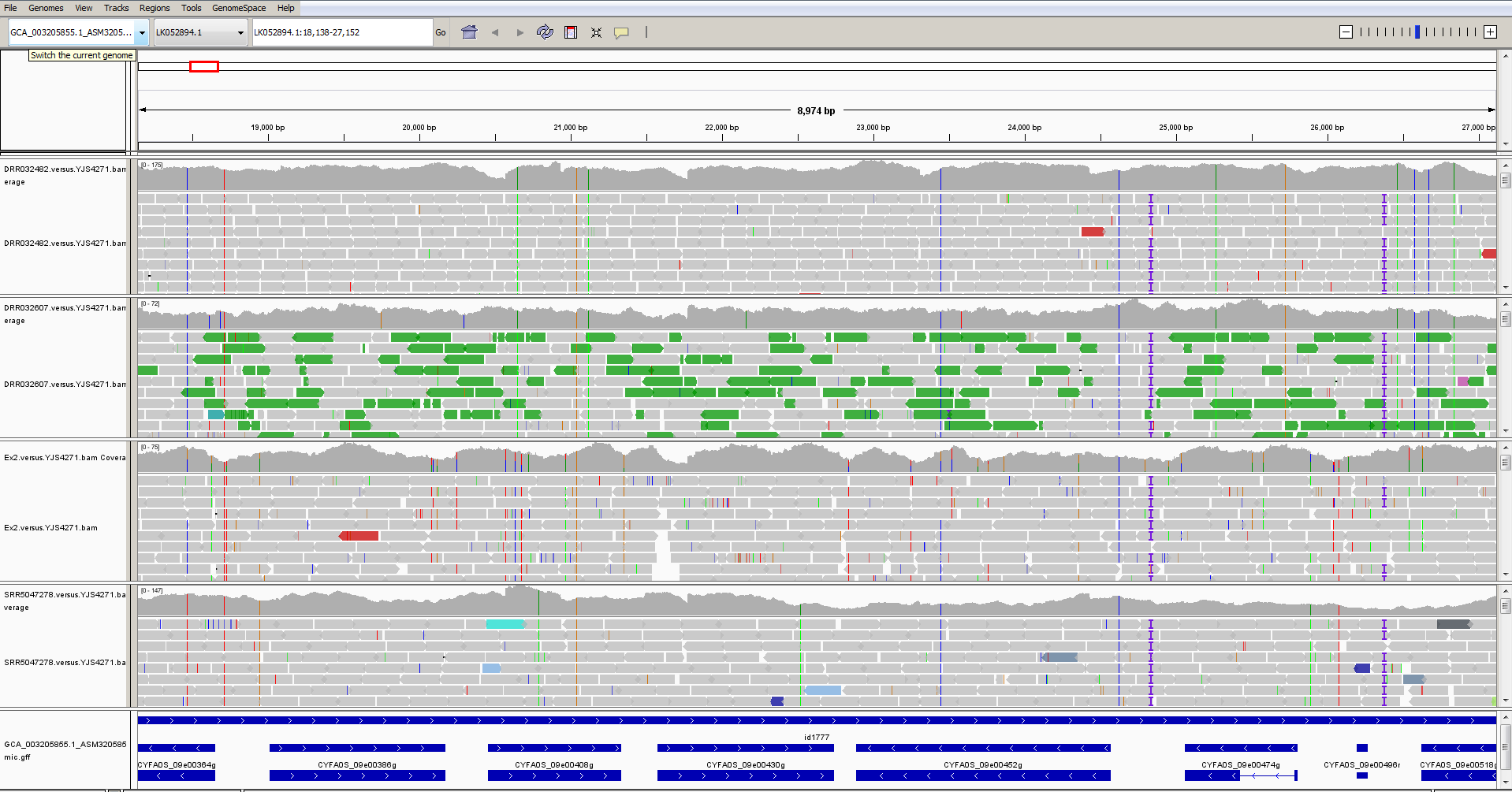
… and after zooming in, it might look something like this:
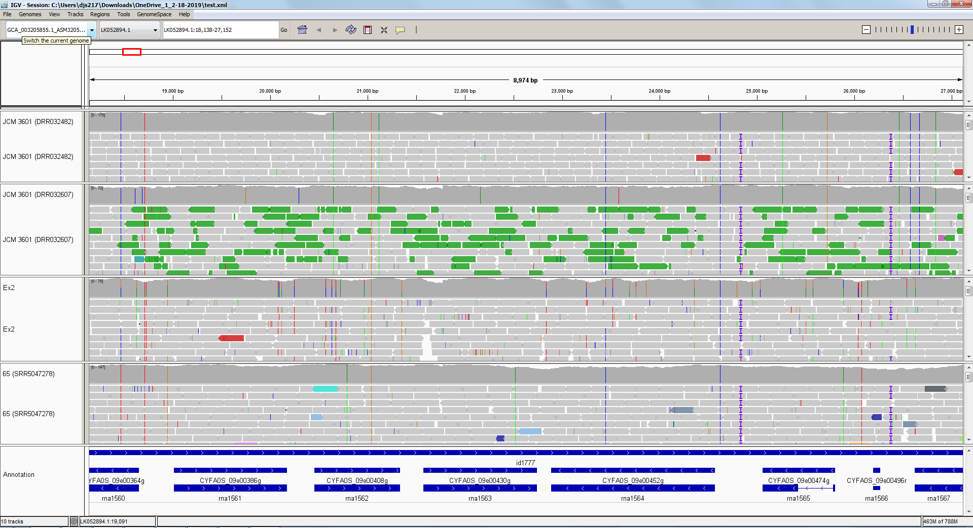
And after right-clicking to rename the tracks and change font sizes, etc., it might look like this:
Now, let’s zoom-in on one of the sequence discrepancies:
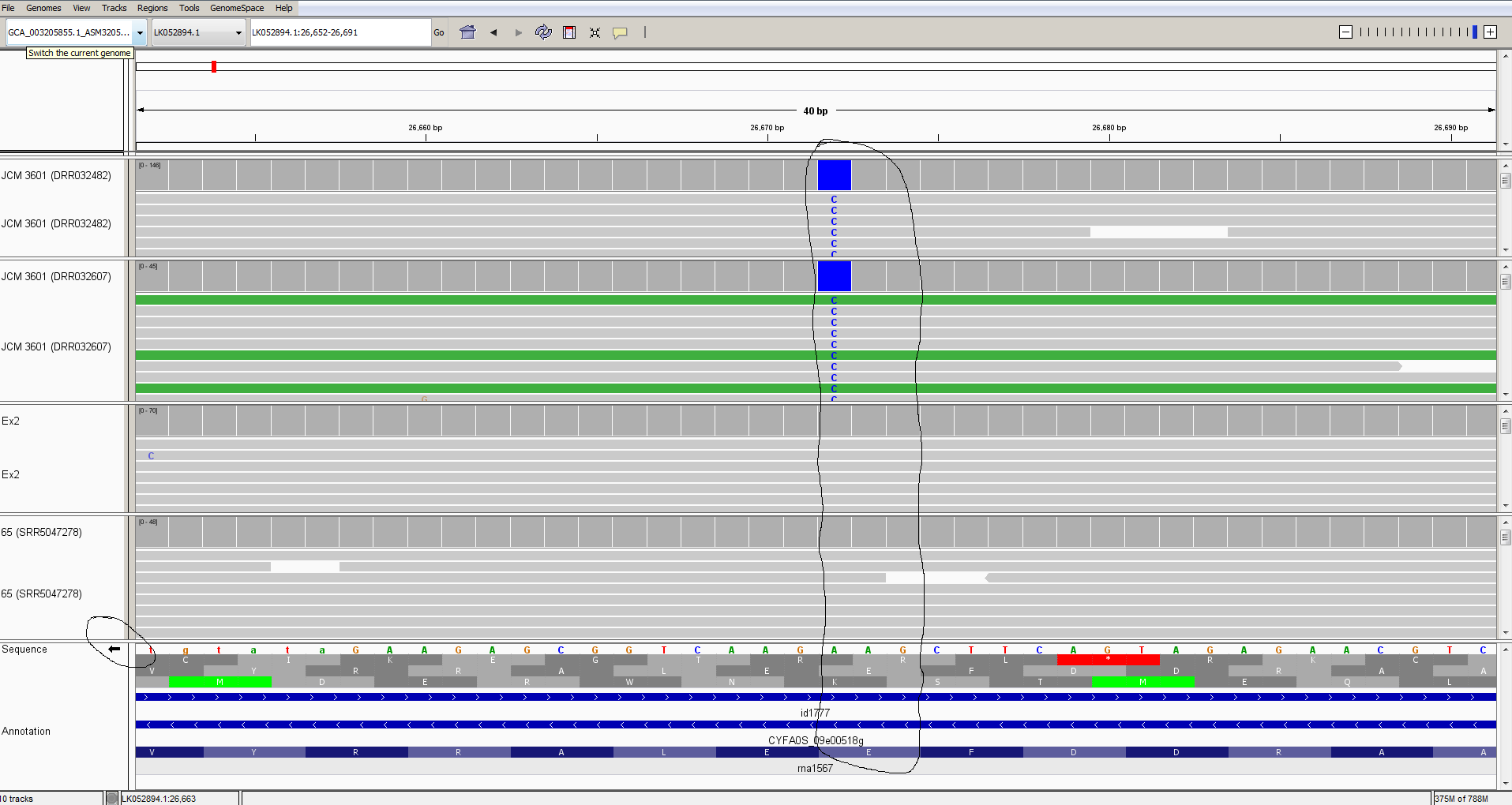
Here we can see a single-nucleotide polymorphism at position LK052894.1:26,672. In strain JCM 3601 there is a C while in genomic reads from strains Ex2 and 65, the reads all agree with the T found in the strain YJS4271 reference sequence.
This polymorphism falls within a GAA codon that encodes glutamate (=E = Glu); in strain JCM 3601, the GAA is changed to GAG, which also encodes glutamate. So, this is a synonymous change that does not affect the amino-acid sequence of the protein.
Note that I have clicked the small arrow at the bottom left to reveal the bases on the reverse strand of the DNA (because this gene happens to be on the reverse strand).
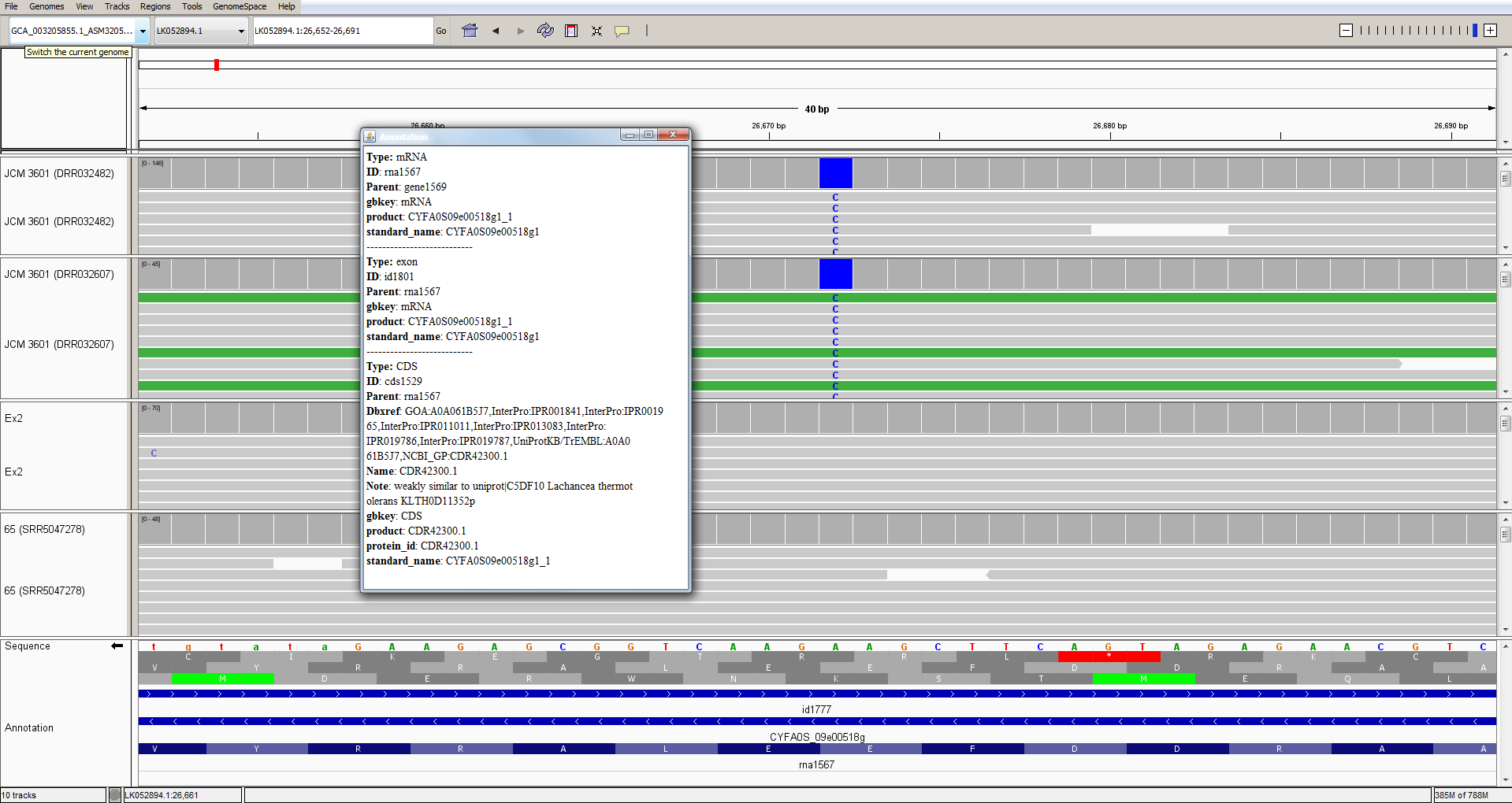
By clicking on the protein sequence, we can obtain a pop-up window with some information about the mutated gene:
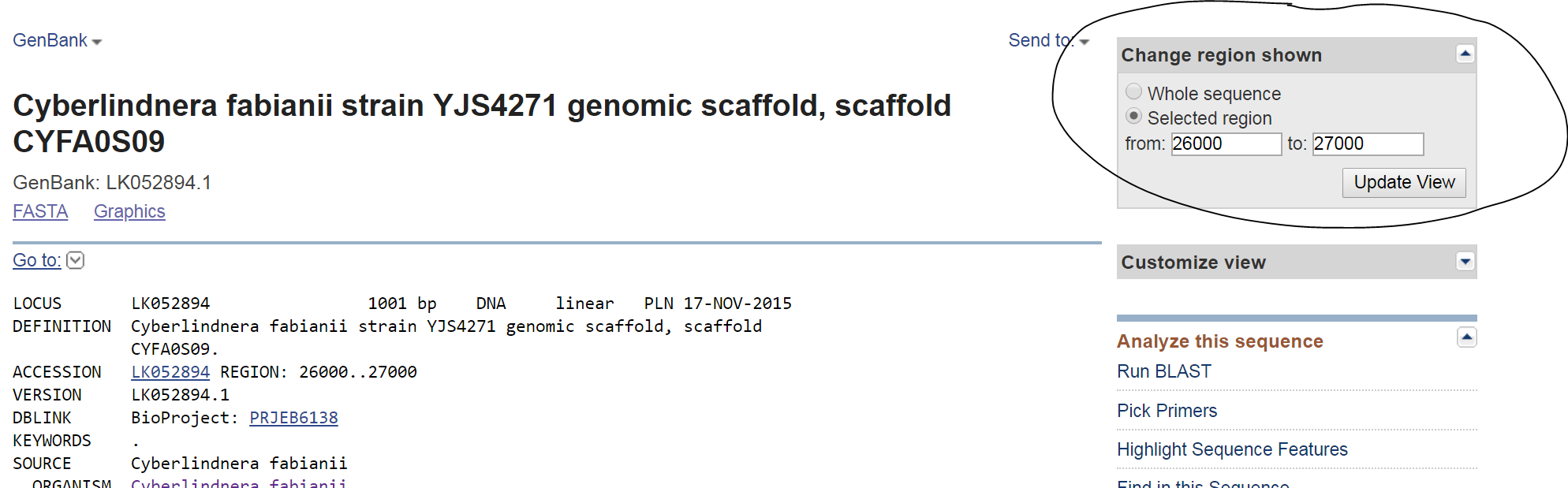
Remember that we can access public sequences via the NCBI Entrez web portal and that we can even access sub-sequences from a larger sequence. So, we could access the sequence of the region that we are looking at here: https://www.ncbi.nlm.nih.gov/nuccore/LK052894.1
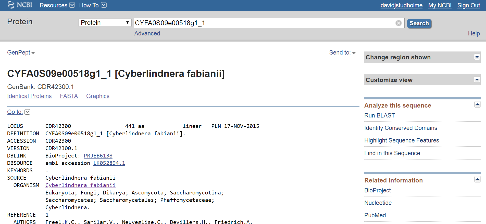
And we can access the protein sequence here: https://www.ncbi.nlm.nih.gov/protein/663445730
Finally, some possible questions that you might consider tackling:
- How different is the Ex2 clinical isolate from previously sequenced non-clinical isolates?
- Can you find any genes that are unusually variable between strains of C. fabianii?
- Are any C. fabianii genes absent from any of the strains?
- Apart from single-nucleotide polymorphisms, can you find any other types of variation?
- Is variation more common in some parts of the genome than others?
- Can you find any loss-of-function mutations?
- To which of the previously sequenced strains is the clinical isolate Ex2 most closely related?
- Are there any genes missing from the annotations?
4.3 Using the web-based version of IGV
If you encounter problems with the locally installed version of IGV, try the web-based version instead.
First, in your web browser, navigate to https://igv.org/app/
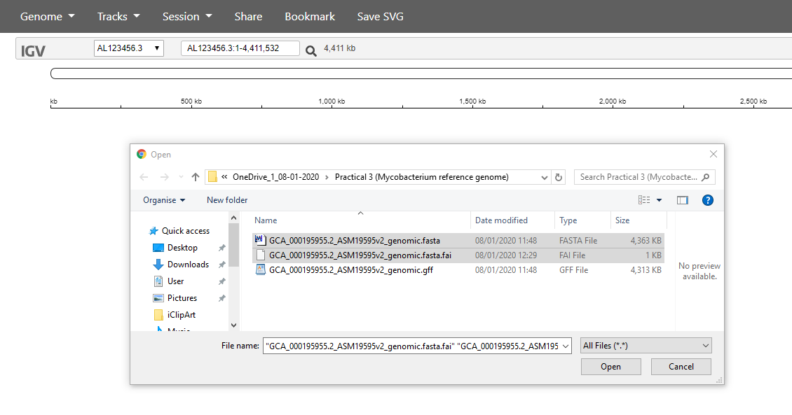
Then use the Genome -> Local File menu item to load your reference genome:
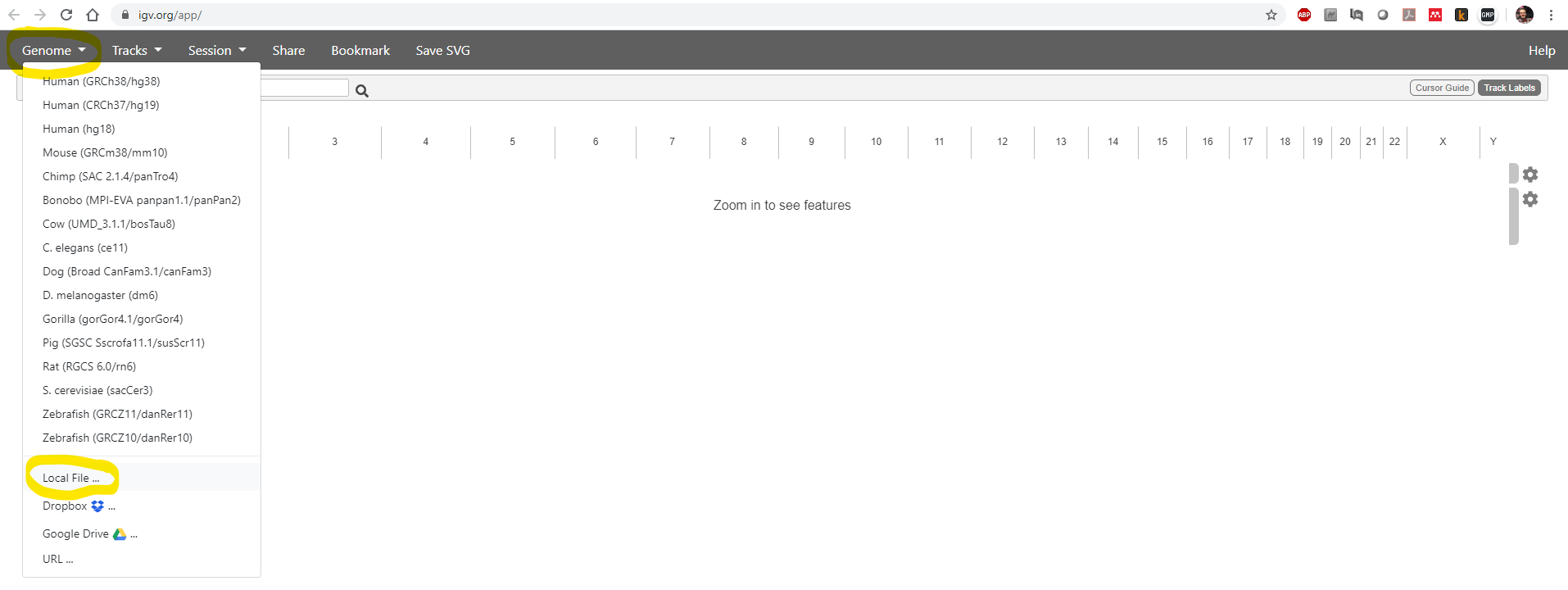
You need to select both of two files: the .fasta sequence file and the .fasta.fai index file:
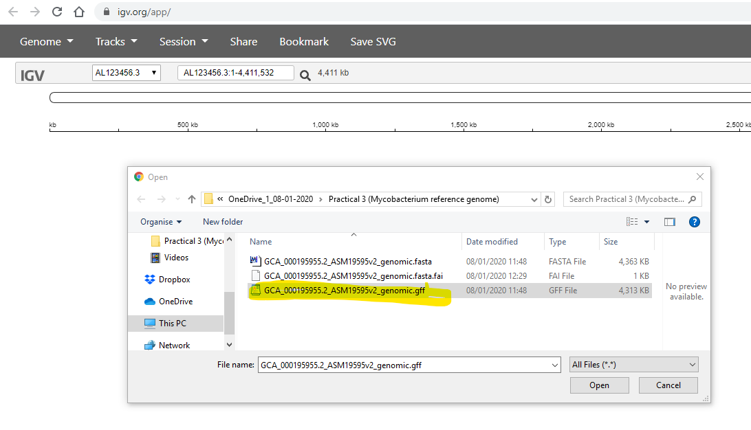
Next, use the Tracks -> Local File menu item to load your annotation.
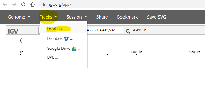
You need to to select the .gff file, which contains the annotation (positions of genes etc) of the reference genome:
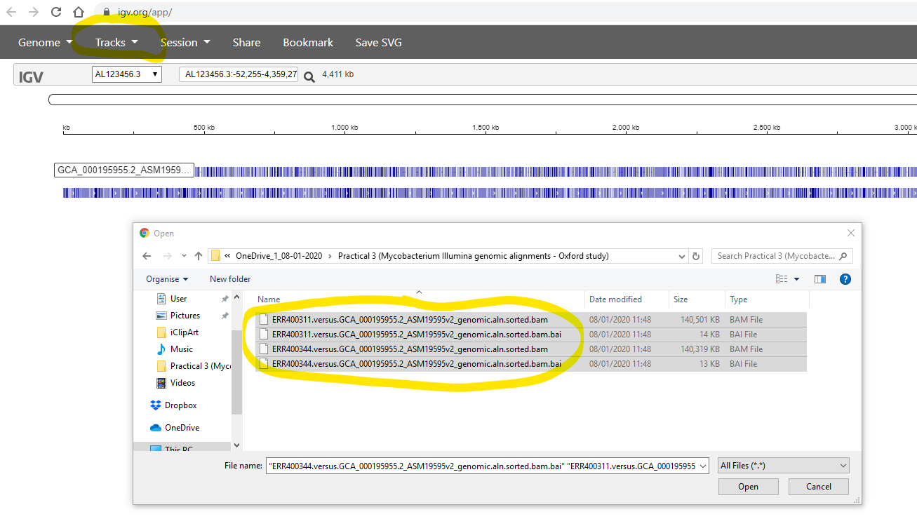
Finally, you use the Tracks -> Local File to select your .bam files. Simultaneously, you also need to select the corrsponding .bam.bai file for each of your .bam files:
After zooming-in (using the tool in the top-right), you should see the aligned reads something like the image below. Note that you can configure various aspects of the display by clicking on the widgets at the right side of the window.