Chapter 7 Wage Analytics
7.1 Introduction
The purpose of this chapter was to create a logistic regression model that predicts wage level (high or low) using factors such as demographics, jobs, and marital status. I ran various tests such as ANOVA, t-test, and chi-square test to help understand and look at the relationships between different variables.
7.2 Creating the WageCategory Variable
##       year           age                     maritl           race                   education
##  Min.   :2003   Min.   :18.00   1. Never Married: 648   1. White:2480   1. < HS Grad      :268
##  1st Qu.:2004   1st Qu.:33.75   2. Married      :2074   2. Black: 293   2. HS Grad        :971
##  Median :2006   Median :42.00   3. Widowed      :  19   3. Asian: 190   3. Some College   :650
##  Mean   :2006   Mean   :42.41   4. Divorced     : 204   4. Other:  37   4. College Grad   :685
##  3rd Qu.:2008   3rd Qu.:51.00   5. Separated    :  55                   5. Advanced Degree:426
##  Max.   :2009   Max.   :80.00
##
##                    region               jobclass               health      health_ins      logwage
##  2. Middle Atlantic   :3000   1. Industrial :1544   1. <=Good     : 858   1. Yes:2083   Min.   :3.000
##  1. New England       :   0   2. Information:1456   2. >=Very Good:2142   2. No : 917   1st Qu.:4.447
##  3. East North Central:   0                                                             Median :4.653
##  4. West North Central:   0                                                             Mean   :4.654
##  5. South Atlantic    :   0                                                             3rd Qu.:4.857
##  6. East South Central:   0                                                             Max.   :5.763
##  (Other)              :   0
##       wage
##  Min.   : 20.09
##  1st Qu.: 85.38
##  Median :104.92
##  Mean   :111.70
##  3rd Qu.:128.68
##  Max.   :318.34
## ## [1] 104.92157.4 Classical Statistical Tests
7.4.1 T-test
##
##  Welch Two Sample t-test
##
## data:  age by WageCategory
## t = -10.888, df = 2855, p-value < 2.2e-16
## alternative hypothesis: true difference in means between group Low and group High is not equal to 0
## 95 percent confidence interval:
##  -5.298535 -3.681416
## sample estimates:
##  mean in group Low mean in group High
##           40.19512           44.68510
The mean age for Low wage earners is 40.19512, and for High wage earners, it’s 44.68510. The t-statistic is -10.888, the df is 2855, and the p-value is less than 0.05, making it statistically significant. This means that age does differ between wage categories.
7.4.2 Anova
## Call:
##    aov(formula = wage ~ education, data = Wage)
##
## Terms:
##                 education Residuals
## Sum of Squares    1226364   3995721
## Deg. of Freedom         4      2995
##
## Residual standard error: 36.52575
## Estimated effects may be unbalanced## Analysis of Variance Table (Type III SS)
## Model: wage ~ education
##
## SS df MS F PRE p
## ----- --------------- | ----------- ---- ---------- ------- ----- -----
## Model (error reduced) | 1226364.485 4 306591.121 229.806 .2348 .0000
## Error (from model) | 3995721.285 2995 1334.131
## ----- --------------- | ----------- ---- ---------- ------- ----- -----
## Total (empty model) | 5222085.770 2999 1741.276The ANOVA table shows us that the F-statistics is 229.806, the df is 4, and the p-value is less than 0.05, making it statistically significant. This test shows us that there is a statistically significant difference between wage and education.
7.4.3 Chi-Square Tests
##
##                    1. < HS Grad 2. HS Grad 3. Some College 4. College Grad 5. Advanced Degree
##   20.0855369231877            0          0               1               0                  0
##   20.9343779401018            1          0               0               0                  0
##   22.9624006796429            0          0               1               0                  0
##   23.2747040516601            0          1               0               0                  0
##   23.9529444789965            0          1               1               0                  0
##   25.2910080971035            0          0               1               0                  0
##   27.1405792079024            1          2               1               0                  0
##   29.3769761006037            0          1               0               0                  0
##   30.9237526933873            0          0               1               0                  0
## 31.4109962716359 0 1 0 0 0##
## Pearson's Chi-squared test
##
## data: wage_cont_table
## X-squared = 2848.6, df = 2028, p-value < 2.2e-16## Cramer V
## 0.4872The x^2 is 2848.6, the df is 2028, the p-value is less than 0.05, showing that the relationship is statistically significant. The Cramer’s V is 0.4872, meaning that there is a moderate effect size between the relationship with wage and marital status.
7.5 Logistic Regression Model
library(caTools)
wage_sample<- sample.split(Wage$WageCategory, SplitRatio= 0.7)
wage_training_data<- subset(Wage, sample=T)
wage_testing_data<- subset(Wage, sample=F)
wage_model<- glm(WageCategory ~ education + age + jobclass + maritl,
                 family= "binomial", data=wage_training_data)
summary(wage_model)
##
## Call:
## glm(formula = WageCategory ~ education + age + jobclass + maritl,
## family = "binomial", data = wage_training_data)
##
## Coefficients:
## Estimate Std. Error z value Pr(>|z|)
## (Intercept) -3.485389 0.243052 -14.340 < 2e-16 ***
## education2. HS Grad 0.788268 0.180789 4.360 1.30e-05 ***
## education3. Some College 1.594690 0.186577 8.547 < 2e-16 ***
## education4. College Grad 2.364116 0.189110 12.501 < 2e-16 ***
## education5. Advanced Degree 3.162107 0.218736 14.456 < 2e-16 ***
## age 0.019705 0.004127 4.774 1.81e-06 ***
## jobclass2. Information 0.238834 0.086978 2.746 0.00603 **
## maritl2. Married 1.246406 0.119553 10.426 < 2e-16 ***
## maritl3. Widowed 0.572058 0.541199 1.057 0.29050
## maritl4. Divorced 0.560192 0.194144 2.885 0.00391 **
## maritl5. Separated 0.600632 0.333203 1.803 0.07145 .
## ---
## Signif. codes: 0 '***' 0.001 '**' 0.01 '*' 0.05 '.' 0.1 ' ' 1
##
## (Dispersion parameter for binomial family taken to be 1)
##
## Null deviance: 4158.5 on 2999 degrees of freedom
## Residual deviance: 3348.2 on 2989 degrees of freedom
## AIC: 3370.2
##
## Number of Fisher Scoring iterations: 4## (Intercept) education2. HS Grad education3. Some College education4. College Grad
## 0.03064184 2.19958409 4.92680116 10.63463642
## education5. Advanced Degree age jobclass2. Information maritl2. Married
## 23.62030034 1.01990027 1.26976776 3.47782266
## maritl3. Widowed maritl4. Divorced maritl5. Separated
## 1.77191052 1.75100794 1.82327070## fitting null model for pseudo-r2## McFadden
## 0.1948651## Overall
## education5. Advanced Degree 14.456240
## education4. College Grad 12.501249
## maritl2. Married 10.425592
## education3. Some College 8.547101
## age 4.774086
## education2. HS Grad 4.360154
## maritl4. Divorced 2.885442
## jobclass2. Information 2.745914
## maritl5. Separated 1.802599
## maritl3. Widowed 1.057020This regression model conveys that Hs Grad, Some College, College Grad, Advanced Degree, age, and married individuals are statistically significant when looking at the relationship with WageCategory. Jobclass isn’t statistically signficant when looking at its relationship with WageCategory. Looking at the odds ratios, we can see that individuals who are college grads for example, have 10.63x the odds of having a high or low wage. One surprising result is the odd ratio for Advanced Degree, which is 23.62, making it the largest ratio among the variables. Looking at the “McFadden”, we can see that this model is kind of weak (0.195) and doesn’t explain a lot of variation. We can also see that education, specifically Advanced Degree is the most impactful variable.
7.6 Model Evaluation
wage_testing_data$pred_prob<- predict(wage_model, newdata = wage_testing_data, type = "response")
wage_testing_data$pred_class<- ifelse(wage_testing_data$pred_prob > 0.5, "High", "Low") %>% as.factor()
View(wage_testing_data)

library(car)
library(caret)
confusionMatrix(wage_testing_data$pred_class, wage_testing_data$WageCategory)
## Confusion Matrix and Statistics
##
## Reference
## Prediction Low High
## Low 1136 471
## High 381 1012
##
## Accuracy : 0.716
## 95% CI : (0.6995, 0.7321)
## No Information Rate : 0.5057
## P-Value [Acc > NIR] : < 2.2e-16
##
## Kappa : 0.4315
##
## Mcnemar's Test P-Value : 0.002295
##
## Sensitivity : 0.7488
## Specificity : 0.6824
## Pos Pred Value : 0.7069
## Neg Pred Value : 0.7265
## Prevalence : 0.5057
## Detection Rate : 0.3787
## Detection Prevalence : 0.5357
## Balanced Accuracy : 0.7156
##
## 'Positive' Class : Low
## library(pROC)
roc_wage<- roc(wage_testing_data$WageCategory, wage_testing_data$pred_prob, levels= c("High", "Low"))
roc_wage##
## Call:
## roc.default(response = wage_testing_data$WageCategory, predictor = wage_testing_data$pred_prob, levels = c("High", "Low"))
##
## Data: wage_testing_data$pred_prob in 1483 controls (wage_testing_data$WageCategory High) > 1517 cases (wage_testing_data$WageCategory Low).
## Area under the curve: 0.7838## Area under the curve: 0.7838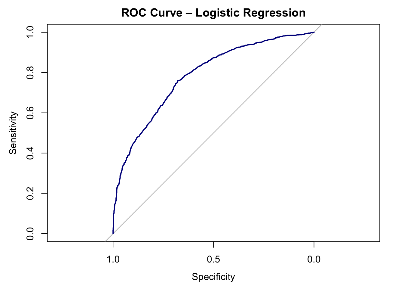
After computing the predicted probabilities and classes and confusion matrix, we can see that the accuracy is 68.67%, the sensitivity is 67.53%, the specificity is 69.86%, and the balanced accuracy is 68.70%. The AUC value is 0.7795, which is good. Our model is also statistically significant.
7.7 Final Interpretation
A logistic regression was conducted to examine whether variables such as age, jobclass, education, or marital status predicted wage level (High or Low). The model was statistically significant, with an accuracy of 68.67%. Our findings convey that education relates to wage the most, and is also a significant predictor in the logistic regression. Married marital status is also significant predictor in the logistic regression. This model best predicts the low wage group. If I repeated this analysis, I would remove the jobclass variable.