Chapter 5 Florida Crime Analytics
5.1 Introduction
The purpose of this chapter was to examine crime in Florida. I looked at 3 variables; income, education, and urbanization to see which one plays the largest role in explaining the differences in crime rates.
5.2 Loading and Preparing the Data
library(readxl)
library(tidyverse)
library(dplyr)


florida_crime<- read_xlsx("Florida County Crime Rates.xlsx")
View(florida_crime)

florida_crime<- florida_crime %>% rename(Crime = C, Income= I, HighSchoolGrad = HS, UrbanPop = U)

florida_crime$County<- str_to_title(florida_crime$County)

str(florida_crime)
## tibble [67 × 5] (S3: tbl_df/tbl/data.frame)
## $ County : chr [1:67] "Alachua" "Baker" "Bay" "Bradford" ...
## $ Crime : num [1:67] 104 20 64 50 64 94 8 35 27 41 ...
## $ Income : num [1:67] 22.1 25.8 24.7 24.6 30.5 30.6 18.6 25.7 21.3 34.9 ...
## $ HighSchoolGrad: num [1:67] 82.7 64.1 74.7 65 82.3 76.8 55.9 75.7 68.6 81.2 ...
## $ UrbanPop : num [1:67] 73.2 21.5 85 23.2 91.9 98.9 0 80.2 31 65.8 ...5.3 Exploratory Data Analysis
##     County              Crime           Income      HighSchoolGrad     UrbanPop
##  Length:67          Min.   :  0.0   Min.   :15.40   Min.   :54.50   Min.   : 0.00
##  Class :character   1st Qu.: 35.5   1st Qu.:21.05   1st Qu.:62.45   1st Qu.:21.60
##  Mode  :character   Median : 52.0   Median :24.60   Median :69.00   Median :44.60
##                     Mean   : 52.4   Mean   :24.51   Mean   :69.49   Mean   :49.56
##                     3rd Qu.: 69.0   3rd Qu.:28.15   3rd Qu.:76.90   3rd Qu.:83.55
## Max. :128.0 Max. :35.60 Max. :84.90 Max. :99.60scatter_florida<- ggplot(florida_crime, aes(x=Income, y=Crime)) +
geom_point()+
labs(
title = "Income and Crime",
x = "Income",
y="Crime"
)
theme.mosaic()## $background
## $background$col
## [1] "transparent"
##
##
## $plot.polygon
## $plot.polygon$col
## [1] "#7171B8"
##
##
## $superpose.polygon
## $superpose.polygon$col
## [1] "#38389C" "lightskyblue3" "darkgreen" "tan" "orange" "purple"
## [7] "lightgreen"
##
##
## $box.rectangle
## $box.rectangle$col
## [1] "#1C1C8E"
##
##
## $box.umbrella
## $box.umbrella$col
## [1] "#1C1C8E"
##
##
## $dot.line
## $dot.line$col
## [1] "#e8e8e8"
##
##
## $dot.symbol
## $dot.symbol$col
## [1] "#1C1C8E"
##
## $dot.symbol$pch
## [1] 16
##
##
## $plot.line
## $plot.line$lwd
## [1] 2
##
## $plot.line$col
## [1] "#1C1C8E"
##
##
## $plot.symbol
## $plot.symbol$col
## [1] "#1C1C8E"
##
## $plot.symbol$pch
## [1] 16
##
##
## $regions
## $regions$col
## [1] "#FF0000" "#FF0300" "#FF0700" "#FF0A00" "#FF0E00" "#FF1100" "#FF1500" "#FF1800" "#FF1C00" "#FF1F00"
## [11] "#FF2200" "#FF2600" "#FF2900" "#FF2D00" "#FF3000" "#FF3400" "#FF3700" "#FF3B00" "#FF3E00" "#FF4100"
## [21] "#FF4500" "#FF4800" "#FF4C00" "#FF4F00" "#FF5300" "#FF5600" "#FF5A00" "#FF5D00" "#FF6000" "#FF6400"
## [31] "#FF6700" "#FF6B00" "#FF6E00" "#FF7200" "#FF7500" "#FF7900" "#FF7C00" "#FF8000" "#FF8300" "#FF8600"
## [41] "#FF8A00" "#FF8D00" "#FF9100" "#FF9400" "#FF9800" "#FF9B00" "#FF9F00" "#FFA200" "#FFA500" "#FFA900"
## [51] "#FFAC00" "#FFB000" "#FFB300" "#FFB700" "#FFBA00" "#FFBE00" "#FFC100" "#FFC400" "#FFC800" "#FFCB00"
## [61] "#FFCF00" "#FFD200" "#FFD600" "#FFD900" "#FFDD00" "#FFE000" "#FFE300" "#FFE700" "#FFEA00" "#FFEE00"
## [71] "#FFF100" "#FFF500" "#FFF800" "#FFFC00" "#FFFF00" "#FFFF05" "#FFFF0F" "#FFFF19" "#FFFF24" "#FFFF2E"
## [81] "#FFFF38" "#FFFF42" "#FFFF4D" "#FFFF57" "#FFFF61" "#FFFF6B" "#FFFF75" "#FFFF80" "#FFFF8A" "#FFFF94"
## [91] "#FFFF9E" "#FFFFA8" "#FFFFB3" "#FFFFBD" "#FFFFC7" "#FFFFD1" "#FFFFDB" "#FFFFE6" "#FFFFF0" "#FFFFFA"
##
##
## $reference.line
## $reference.line$col
## [1] "#e8e8e8"
##
##
## $add.line
## $add.line$lty
## [1] 1
##
## $add.line$col
## [1] "gray20"
##
## $add.line$lwd
## [1] 2
##
##
## $superpose.line
## $superpose.line$lty
## [1] 1
##
## $superpose.line$col
## [1] "#1C1C8E" "lightskyblue3" "darkgreen" "tan" "orange" "purple"
## [7] "pink" "lightgreen"
##
##
## $superpose.symbol
## $superpose.symbol$pch
## [1] 16 15 18 1 3 6 0 5
##
## $superpose.symbol$cex
## [1] 0.7 0.7 0.7 0.7 0.7 0.7 0.7
##
## $superpose.symbol$col
## [1] "#1C1C8E" "lightskyblue3" "darkgreen" "tan" "orange" "purple"
## [7] "pink" "lightgreen"
##
##
## $strip.background
## $strip.background$alpha
## [1] 1
##
## $strip.background$col
## [1] "#ffe5cc" "#DDE8F1" "#ccffff" "#cce6ff" "#ffccff" "#ffcccc" "#ffffcc"
##
##
## $strip.shingle
## $strip.shingle$alpha
## [1] 1
##
## $strip.shingle$col
## [1] "#ff7f00" "#1C1C8E" "#00ffff" "#0080ff" "#ff00ff" "#ff0000" "#ffff00"
##
##
## $par.strip.text
## $par.strip.text$cex
## [1] 0.5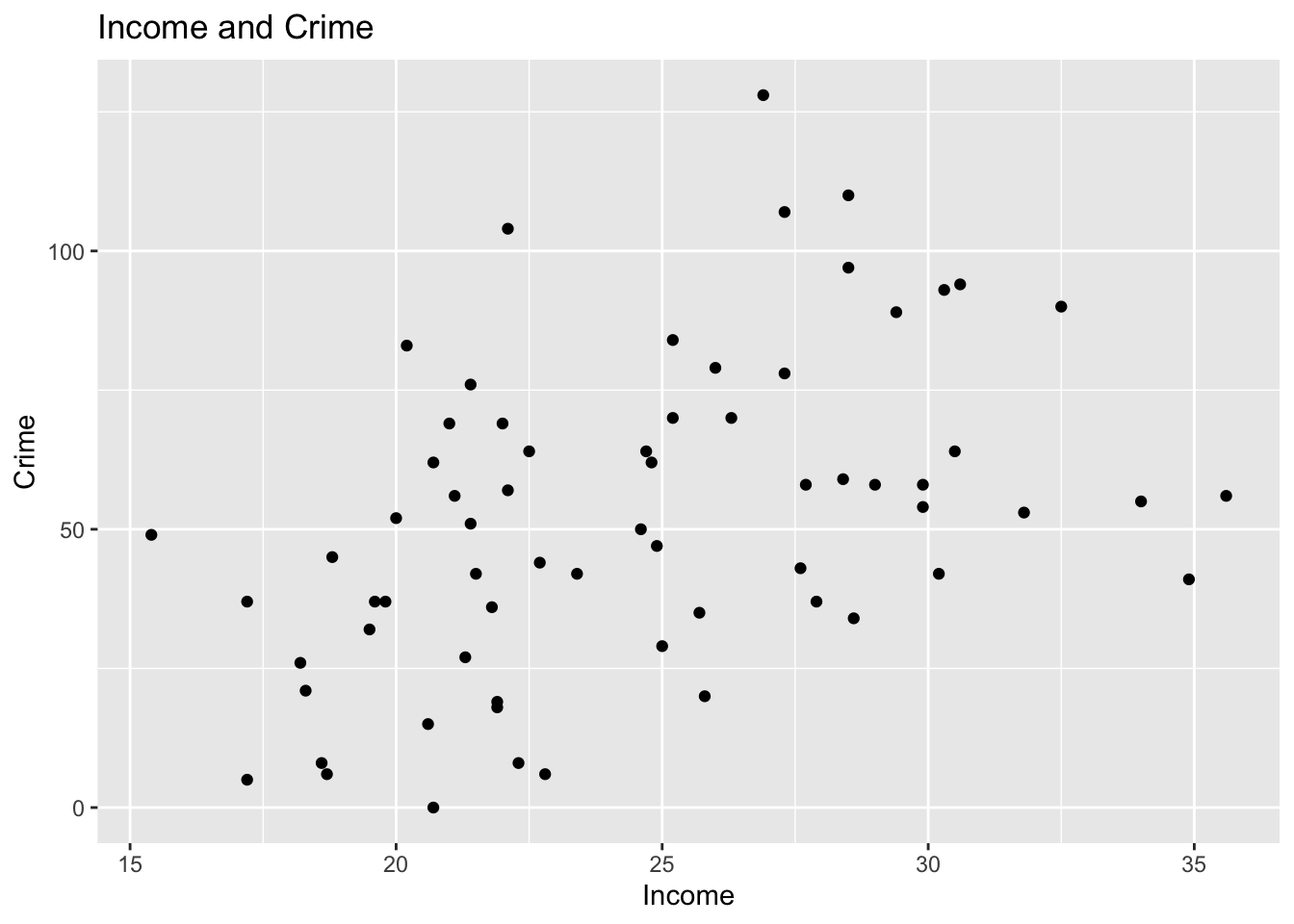
Figure 5.1: This scatter plot looks at the relationship between crime and income in Florida.
This scatterplot conveys that as the Income increases, the crime rate slowly increases as well.
hist_florida<- ggplot(florida_crime, aes(x=Income)) +
  geom_histogram()+
  labs(
    title = "Florida Income",
    x = "Income",
    y = "Count"
  )
theme_minimal()
## <theme> List of 144
## $ line : <ggplot2::element_line>
## ..@ colour : chr "black"
## ..@ linewidth : num 0.5
## ..@ linetype : num 1
## ..@ lineend : chr "butt"
## ..@ linejoin : chr "round"
## ..@ arrow : logi FALSE
## ..@ arrow.fill : chr "black"
## ..@ inherit.blank: logi TRUE
## $ rect : <ggplot2::element_rect>
## ..@ fill : chr "white"
## ..@ colour : chr "black"
## ..@ linewidth : num 0.5
## ..@ linetype : num 1
## ..@ linejoin : chr "round"
## ..@ inherit.blank: logi TRUE
## $ text : <ggplot2::element_text>
## ..@ family : chr ""
## ..@ face : chr "plain"
## ..@ italic : chr NA
## ..@ fontweight : num NA
## ..@ fontwidth : num NA
## ..@ colour : chr "black"
## ..@ size : num 11
## ..@ hjust : num 0.5
## ..@ vjust : num 0.5
## ..@ angle : num 0
## ..@ lineheight : num 0.9
## ..@ margin : <ggplot2::margin> num [1:4] 0 0 0 0
## ..@ debug : logi FALSE
## ..@ inherit.blank: logi TRUE
## $ title : <ggplot2::element_text>
## ..@ family : NULL
## ..@ face : NULL
## ..@ italic : chr NA
## ..@ fontweight : num NA
## ..@ fontwidth : num NA
## ..@ colour : NULL
## ..@ size : NULL
## ..@ hjust : NULL
## ..@ vjust : NULL
## ..@ angle : NULL
## ..@ lineheight : NULL
## ..@ margin : NULL
## ..@ debug : NULL
## ..@ inherit.blank: logi TRUE
## $ point : <ggplot2::element_point>
## ..@ colour : chr "black"
## ..@ shape : num 19
## ..@ size : num 1.5
## ..@ fill : chr "white"
## ..@ stroke : num 0.5
## ..@ inherit.blank: logi TRUE
## $ polygon : <ggplot2::element_polygon>
## ..@ fill : chr "white"
## ..@ colour : chr "black"
## ..@ linewidth : num 0.5
## ..@ linetype : num 1
## ..@ linejoin : chr "round"
## ..@ inherit.blank: logi TRUE
## $ geom : <ggplot2::element_geom>
## ..@ ink : chr "black"
## ..@ paper : chr "white"
## ..@ accent : chr "#3366FF"
## ..@ linewidth : num 0.5
## ..@ borderwidth: num 0.5
## ..@ linetype : int 1
## ..@ bordertype : int 1
## ..@ family : chr ""
## ..@ fontsize : num 3.87
## ..@ pointsize : num 1.5
## ..@ pointshape : num 19
## ..@ colour : NULL
## ..@ fill : NULL
## $ spacing : 'simpleUnit' num 5.5points
## ..- attr(*, "unit")= int 8
## $ margins : <ggplot2::margin> num [1:4] 5.5 5.5 5.5 5.5
## $ aspect.ratio : NULL
## $ axis.title : NULL
## $ axis.title.x : <ggplot2::element_text>
## ..@ family : NULL
## ..@ face : NULL
## ..@ italic : chr NA
## ..@ fontweight : num NA
## ..@ fontwidth : num NA
## ..@ colour : NULL
## ..@ size : NULL
## ..@ hjust : NULL
## ..@ vjust : num 1
## ..@ angle : NULL
## ..@ lineheight : NULL
## ..@ margin : <ggplot2::margin> num [1:4] 2.75 0 0 0
## ..@ debug : NULL
## ..@ inherit.blank: logi TRUE
## $ axis.title.x.top : <ggplot2::element_text>
## ..@ family : NULL
## ..@ face : NULL
## ..@ italic : chr NA
## ..@ fontweight : num NA
## ..@ fontwidth : num NA
## ..@ colour : NULL
## ..@ size : NULL
## ..@ hjust : NULL
## ..@ vjust : num 0
## ..@ angle : NULL
## ..@ lineheight : NULL
## ..@ margin : <ggplot2::margin> num [1:4] 0 0 2.75 0
## ..@ debug : NULL
## ..@ inherit.blank: logi TRUE
## $ axis.title.x.bottom : NULL
## $ axis.title.y : <ggplot2::element_text>
## ..@ family : NULL
## ..@ face : NULL
## ..@ italic : chr NA
## ..@ fontweight : num NA
## ..@ fontwidth : num NA
## ..@ colour : NULL
## ..@ size : NULL
## ..@ hjust : NULL
## ..@ vjust : num 1
## ..@ angle : num 90
## ..@ lineheight : NULL
## ..@ margin : <ggplot2::margin> num [1:4] 0 2.75 0 0
## ..@ debug : NULL
## ..@ inherit.blank: logi TRUE
## $ axis.title.y.left : NULL
## $ axis.title.y.right : <ggplot2::element_text>
## ..@ family : NULL
## ..@ face : NULL
## ..@ italic : chr NA
## ..@ fontweight : num NA
## ..@ fontwidth : num NA
## ..@ colour : NULL
## ..@ size : NULL
## ..@ hjust : NULL
## ..@ vjust : num 1
## ..@ angle : num -90
## ..@ lineheight : NULL
## ..@ margin : <ggplot2::margin> num [1:4] 0 0 0 2.75
## ..@ debug : NULL
## ..@ inherit.blank: logi TRUE
## $ axis.text : <ggplot2::element_text>
## ..@ family : NULL
## ..@ face : NULL
## ..@ italic : chr NA
## ..@ fontweight : num NA
## ..@ fontwidth : num NA
## ..@ colour : chr "#4D4D4DFF"
## ..@ size : 'rel' num 0.8
## ..@ hjust : NULL
## ..@ vjust : NULL
## ..@ angle : NULL
## ..@ lineheight : NULL
## ..@ margin : NULL
## ..@ debug : NULL
## ..@ inherit.blank: logi TRUE
## $ axis.text.x : <ggplot2::element_text>
## ..@ family : NULL
## ..@ face : NULL
## ..@ italic : chr NA
## ..@ fontweight : num NA
## ..@ fontwidth : num NA
## ..@ colour : NULL
## ..@ size : NULL
## ..@ hjust : NULL
## ..@ vjust : num 1
## ..@ angle : NULL
## ..@ lineheight : NULL
## ..@ margin : <ggplot2::margin> num [1:4] 2.2 0 0 0
## ..@ debug : NULL
## ..@ inherit.blank: logi TRUE
## $ axis.text.x.top : <ggplot2::element_text>
## ..@ family : NULL
## ..@ face : NULL
## ..@ italic : chr NA
## ..@ fontweight : num NA
## ..@ fontwidth : num NA
## ..@ colour : NULL
## ..@ size : NULL
## ..@ hjust : NULL
## ..@ vjust : NULL
## ..@ angle : NULL
## ..@ lineheight : NULL
## ..@ margin : <ggplot2::margin> num [1:4] 0 0 4.95 0
## ..@ debug : NULL
## ..@ inherit.blank: logi TRUE
## $ axis.text.x.bottom : <ggplot2::element_text>
## ..@ family : NULL
## ..@ face : NULL
## ..@ italic : chr NA
## ..@ fontweight : num NA
## ..@ fontwidth : num NA
## ..@ colour : NULL
## ..@ size : NULL
## ..@ hjust : NULL
## ..@ vjust : NULL
## ..@ angle : NULL
## ..@ lineheight : NULL
## ..@ margin : <ggplot2::margin> num [1:4] 4.95 0 0 0
## ..@ debug : NULL
## ..@ inherit.blank: logi TRUE
## $ axis.text.y : <ggplot2::element_text>
## ..@ family : NULL
## ..@ face : NULL
## ..@ italic : chr NA
## ..@ fontweight : num NA
## ..@ fontwidth : num NA
## ..@ colour : NULL
## ..@ size : NULL
## ..@ hjust : num 1
## ..@ vjust : NULL
## ..@ angle : NULL
## ..@ lineheight : NULL
## ..@ margin : <ggplot2::margin> num [1:4] 0 2.2 0 0
## ..@ debug : NULL
## ..@ inherit.blank: logi TRUE
## $ axis.text.y.left : <ggplot2::element_text>
## ..@ family : NULL
## ..@ face : NULL
## ..@ italic : chr NA
## ..@ fontweight : num NA
## ..@ fontwidth : num NA
## ..@ colour : NULL
## ..@ size : NULL
## ..@ hjust : NULL
## ..@ vjust : NULL
## ..@ angle : NULL
## ..@ lineheight : NULL
## ..@ margin : <ggplot2::margin> num [1:4] 0 4.95 0 0
## ..@ debug : NULL
## ..@ inherit.blank: logi TRUE
## $ axis.text.y.right : <ggplot2::element_text>
## ..@ family : NULL
## ..@ face : NULL
## ..@ italic : chr NA
## ..@ fontweight : num NA
## ..@ fontwidth : num NA
## ..@ colour : NULL
## ..@ size : NULL
## ..@ hjust : NULL
## ..@ vjust : NULL
## ..@ angle : NULL
## ..@ lineheight : NULL
## ..@ margin : <ggplot2::margin> num [1:4] 0 0 0 4.95
## ..@ debug : NULL
## ..@ inherit.blank: logi TRUE
## $ axis.text.theta : NULL
## $ axis.text.r : <ggplot2::element_text>
## ..@ family : NULL
## ..@ face : NULL
## ..@ italic : chr NA
## ..@ fontweight : num NA
## ..@ fontwidth : num NA
## ..@ colour : NULL
## ..@ size : NULL
## ..@ hjust : num 0.5
## ..@ vjust : NULL
## ..@ angle : NULL
## ..@ lineheight : NULL
## ..@ margin : <ggplot2::margin> num [1:4] 0 2.2 0 2.2
## ..@ debug : NULL
## ..@ inherit.blank: logi TRUE
## $ axis.ticks : <ggplot2::element_blank>
## $ axis.ticks.x : NULL
## $ axis.ticks.x.top : NULL
## $ axis.ticks.x.bottom : NULL
## $ axis.ticks.y : NULL
## $ axis.ticks.y.left : NULL
## $ axis.ticks.y.right : NULL
## $ axis.ticks.theta : NULL
## $ axis.ticks.r : NULL
## $ axis.minor.ticks.x.top : NULL
## $ axis.minor.ticks.x.bottom : NULL
## $ axis.minor.ticks.y.left : NULL
## $ axis.minor.ticks.y.right : NULL
## $ axis.minor.ticks.theta : NULL
## $ axis.minor.ticks.r : NULL
## $ axis.ticks.length : 'rel' num 0.5
## $ axis.ticks.length.x : NULL
## $ axis.ticks.length.x.top : NULL
## $ axis.ticks.length.x.bottom : NULL
## $ axis.ticks.length.y : NULL
## $ axis.ticks.length.y.left : NULL
## $ axis.ticks.length.y.right : NULL
## $ axis.ticks.length.theta : NULL
## $ axis.ticks.length.r : NULL
## $ axis.minor.ticks.length : 'rel' num 0.75
## $ axis.minor.ticks.length.x : NULL
## $ axis.minor.ticks.length.x.top : NULL
## $ axis.minor.ticks.length.x.bottom: NULL
## $ axis.minor.ticks.length.y : NULL
## $ axis.minor.ticks.length.y.left : NULL
## $ axis.minor.ticks.length.y.right : NULL
## $ axis.minor.ticks.length.theta : NULL
## $ axis.minor.ticks.length.r : NULL
## $ axis.line : <ggplot2::element_blank>
## $ axis.line.x : NULL
## $ axis.line.x.top : NULL
## $ axis.line.x.bottom : NULL
## $ axis.line.y : NULL
## $ axis.line.y.left : NULL
## $ axis.line.y.right : NULL
## $ axis.line.theta : NULL
## $ axis.line.r : NULL
## $ legend.background : <ggplot2::element_blank>
## $ legend.margin : NULL
## $ legend.spacing : 'rel' num 2
## $ legend.spacing.x : NULL
## $ legend.spacing.y : NULL
## $ legend.key : <ggplot2::element_blank>
## $ legend.key.size : 'simpleUnit' num 1.2lines
## ..- attr(*, "unit")= int 3
## $ legend.key.height : NULL
## $ legend.key.width : NULL
## $ legend.key.spacing : NULL
## $ legend.key.spacing.x : NULL
## $ legend.key.spacing.y : NULL
## $ legend.key.justification : NULL
## $ legend.frame : NULL
## $ legend.ticks : NULL
## $ legend.ticks.length : 'rel' num 0.2
## $ legend.axis.line : NULL
## $ legend.text : <ggplot2::element_text>
## ..@ family : NULL
## ..@ face : NULL
## ..@ italic : chr NA
## ..@ fontweight : num NA
## ..@ fontwidth : num NA
## ..@ colour : NULL
## ..@ size : 'rel' num 0.8
## ..@ hjust : NULL
## ..@ vjust : NULL
## ..@ angle : NULL
## ..@ lineheight : NULL
## ..@ margin : NULL
## ..@ debug : NULL
## ..@ inherit.blank: logi TRUE
## $ legend.text.position : NULL
## $ legend.title : <ggplot2::element_text>
## ..@ family : NULL
## ..@ face : NULL
## ..@ italic : chr NA
## ..@ fontweight : num NA
## ..@ fontwidth : num NA
## ..@ colour : NULL
## ..@ size : NULL
## ..@ hjust : num 0
## ..@ vjust : NULL
## ..@ angle : NULL
## ..@ lineheight : NULL
## ..@ margin : NULL
## ..@ debug : NULL
## ..@ inherit.blank: logi TRUE
## $ legend.title.position : NULL
## $ legend.position : chr "right"
## $ legend.position.inside : NULL
## $ legend.direction : NULL
## $ legend.byrow : NULL
## $ legend.justification : chr "center"
## $ legend.justification.top : NULL
## $ legend.justification.bottom : NULL
## $ legend.justification.left : NULL
## $ legend.justification.right : NULL
## $ legend.justification.inside : NULL
## [list output truncated]
## @ complete: logi TRUE
## @ validate: logi TRUE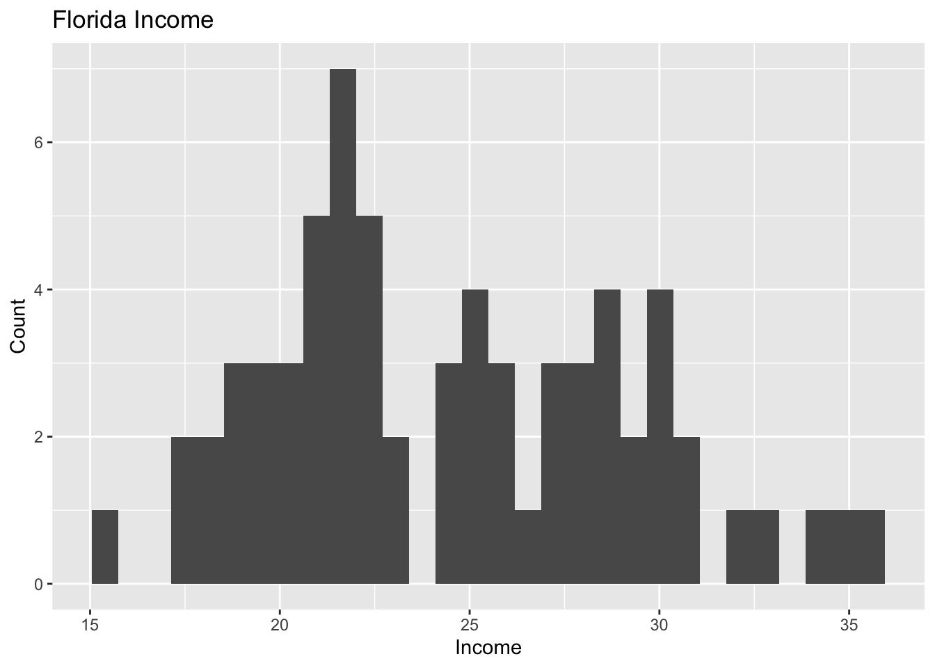
Figure 5.2: This histogram shows the range of individuals incomes in Flordia.
This histogram shows us that many individuals income is between $21,000 - $30,000 in across the state of Florida.
5.4 Correlation Analysis
library(ggcorrplot)
florida_matrix<- florida_crime %>% dplyr::select(Crime, Income, HighSchoolGrad, UrbanPop)
florida_crime_matrix<- cor(florida_matrix, use="pairwise.complete.obs")
florida_crime_matrix
## Crime Income HighSchoolGrad UrbanPop
## Crime 1.0000000 0.4337503 0.4669119 0.6773678
## Income 0.4337503 1.0000000 0.7926215 0.7306983
## HighSchoolGrad 0.4669119 0.7926215 1.0000000 0.7907190
## UrbanPop 0.6773678 0.7306983 0.7907190 1.0000000ggcorrplot(florida_crime_matrix, lab=TRUE, type="lower")+
labs(title="Correlation Matrix: Florida Crime")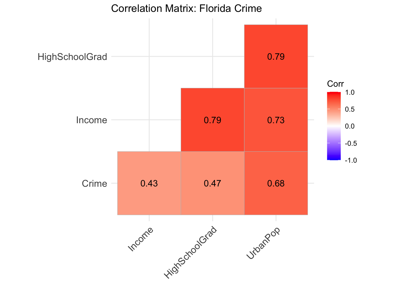
Figure 5.3: This figure is a correlation matrix that shows the relationships between high school graduation rate, income, crime, and urban pop in Florida.
The variable that shows the strongest relationship with Crime is UrbanPop (0.68). All variables have positive relationships, however, some are stronger than others.
The relationship between HighSchoolGrad and UrbanPop is 0.79 which is one of the strongest, positive correlations among all the variables. The relationship between HighSchoolGrad and Income is also 0.79, which makes it another strong, positive correlation.
The relationship between Income and UrbanPop is 0.73, making it another strong, positive correlation. The relationship between Crime and HighSchoolGrad is 0.47, making it a moderate, positive correlation. The relationship between Crime and Income is 0.43, making it another moderate, positive correlation.
5.5 Building Regression Models
##
## Call:
## lm(formula = Crime ~ UrbanPop, data = florida_crime)
##
## Coefficients:
## (Intercept)     UrbanPop
## 24.5412 0.5622##
## Call:
## lm(formula = Crime ~ UrbanPop, data = florida_crime)
##
## Residuals:
## Min 1Q Median 3Q Max
## -34.766 -16.541 -4.741 16.521 49.632
##
## Coefficients:
## Estimate Std. Error t value Pr(>|t|)
## (Intercept) 24.54125 4.53930 5.406 9.85e-07 ***
## UrbanPop 0.56220 0.07573 7.424 3.08e-10 ***
## ---
## Signif. codes: 0 '***' 0.001 '**' 0.01 '*' 0.05 '.' 0.1 ' ' 1
##
## Residual standard error: 20.9 on 65 degrees of freedom
## Multiple R-squared: 0.4588, Adjusted R-squared: 0.4505
## F-statistic: 55.11 on 1 and 65 DF, p-value: 3.084e-10## # A tibble: 2 × 5
## term estimate std.error statistic p.value
## <chr> <dbl> <dbl> <dbl> <dbl>
## 1 (Intercept) 24.5 4.54 5.41 9.85e- 7
## 2 UrbanPop 0.562 0.0757 7.42 3.08e-10##
## Call:
## lm(formula = Crime ~ HighSchoolGrad, data = florida_crime)
##
## Coefficients:
## (Intercept) HighSchoolGrad
## -50.857 1.486##
## Call:
## lm(formula = Crime ~ HighSchoolGrad, data = florida_crime)
##
## Residuals:
## Min 1Q Median 3Q Max
## -43.74 -21.36 -4.82 17.42 82.27
##
## Coefficients:
## Estimate Std. Error t value Pr(>|t|)
## (Intercept) -50.8569 24.4507 -2.080 0.0415 *
## HighSchoolGrad 1.4860 0.3491 4.257 6.81e-05 ***
## ---
## Signif. codes: 0 '***' 0.001 '**' 0.01 '*' 0.05 '.' 0.1 ' ' 1
##
## Residual standard error: 25.12 on 65 degrees of freedom
## Multiple R-squared: 0.218, Adjusted R-squared: 0.206
## F-statistic: 18.12 on 1 and 65 DF, p-value: 6.806e-05## # A tibble: 2 × 5
## term estimate std.error statistic p.value
## <chr> <dbl> <dbl> <dbl> <dbl>
## 1 (Intercept) -50.9 24.5 -2.08 0.0415
## 2 HighSchoolGrad 1.49 0.349 4.26 0.0000681##
## Call:
## lm(formula = Crime ~ Income, data = florida_crime)
##
## Coefficients:
## (Intercept) Income
## -11.606 2.611##
## Call:
## lm(formula = Crime ~ Income, data = florida_crime)
##
## Residuals:
## Min 1Q Median 3Q Max
## -42.452 -21.347 -3.102 17.580 69.357
##
## Coefficients:
## Estimate Std. Error t value Pr(>|t|)
## (Intercept) -11.6059 16.7863 -0.691 0.491782
## Income 2.6115 0.6729 3.881 0.000246 ***
## ---
## Signif. codes: 0 '***' 0.001 '**' 0.01 '*' 0.05 '.' 0.1 ' ' 1
##
## Residual standard error: 25.6 on 65 degrees of freedom
## Multiple R-squared: 0.1881, Adjusted R-squared: 0.1756
## F-statistic: 15.06 on 1 and 65 DF, p-value: 0.0002456## # A tibble: 2 × 5
## term estimate std.error statistic p.value
## <chr> <dbl> <dbl> <dbl> <dbl>
## 1 (Intercept) -11.6 16.8 -0.691 0.492
## 2 Income 2.61 0.673 3.88 0.000246##
## Call:
## lm(formula = Crime ~ Income + HighSchoolGrad, data = florida_crime)
##
## Coefficients:
## (Intercept) Income HighSchoolGrad
## -46.109 1.031 1.054## # A tibble: 1 × 12
## r.squared adj.r.squared sigma statistic p.value df logLik AIC BIC deviance df.residual nobs
## <dbl> <dbl> <dbl> <dbl> <dbl> <dbl> <dbl> <dbl> <dbl> <dbl> <int> <int>
## 1 0.229 0.205 25.1 9.50 0.000244 2 -310. 627. 636. 40453. 64 67## # A tibble: 3 × 5
## term estimate std.error statistic p.value
## <chr> <dbl> <dbl> <dbl> <dbl>
## 1 (Intercept) -46.1 25.0 -1.85 0.0695
## 2 Income 1.03 1.08 0.951 0.345
## 3 HighSchoolGrad 1.05 0.573 1.84 0.0705##
## Call:
## lm(formula = Crime ~ Income + UrbanPop, data = florida_crime)
##
## Coefficients:
## (Intercept) Income UrbanPop
## 39.9723 -0.7906 0.6418## # A tibble: 1 × 12
## r.squared adj.r.squared sigma statistic p.value df logLik AIC BIC deviance df.residual nobs
## <dbl> <dbl> <dbl> <dbl> <dbl> <dbl> <dbl> <dbl> <dbl> <dbl> <int> <int>
## 1 0.467 0.450 20.9 28.0 0.00000000181 2 -297. 602. 611. 27969. 64 67## # A tibble: 3 × 5
## term estimate std.error statistic p.value
## <chr> <dbl> <dbl> <dbl> <dbl>
## 1 (Intercept) 40.0 16.4 2.44 0.0173
## 2 Income -0.791 0.805 -0.982 0.330
## 3 UrbanPop 0.642 0.111 5.78 0.000000236##
## Call:
## lm(formula = Crime ~ HighSchoolGrad + Income + UrbanPop, data = florida_crime)
##
## Coefficients:
## (Intercept) HighSchoolGrad Income UrbanPop
## 59.7147 -0.4673 -0.3831 0.6972## # A tibble: 1 × 12
## r.squared adj.r.squared sigma statistic p.value df logLik AIC BIC deviance df.residual nobs
## <dbl> <dbl> <dbl> <dbl> <dbl> <dbl> <dbl> <dbl> <dbl> <dbl> <int> <int>
## 1 0.473 0.448 21.0 18.8 0.00000000782 3 -297. 604. 615. 27658. 63 67## # A tibble: 4 × 5
## term estimate std.error statistic p.value
## <chr> <dbl> <dbl> <dbl> <dbl>
## 1 (Intercept) 59.7 28.6 2.09 0.0408
## 2 HighSchoolGrad -0.467 0.554 -0.843 0.403
## 3 Income -0.383 0.941 -0.407 0.685
## 4 UrbanPop 0.697 0.129 5.40 0.00000108##
## Call:
## lm(formula = Crime ~ UrbanPop + HighSchoolGrad, data = florida_crime)
##
## Coefficients:
## (Intercept) UrbanPop HighSchoolGrad
## 59.1181 0.6825 -0.5834##
## Call:
## lm(formula = Crime ~ UrbanPop + HighSchoolGrad, data = florida_crime)
##
## Residuals:
## Min 1Q Median 3Q Max
## -34.693 -15.742 -6.226 15.812 50.678
##
## Coefficients:
## Estimate Std. Error t value Pr(>|t|)
## (Intercept) 59.1181 28.3653 2.084 0.0411 *
## UrbanPop 0.6825 0.1232 5.539 6.11e-07 ***
## HighSchoolGrad -0.5834 0.4725 -1.235 0.2214
## ---
## Signif. codes: 0 '***' 0.001 '**' 0.01 '*' 0.05 '.' 0.1 ' ' 1
##
## Residual standard error: 20.82 on 64 degrees of freedom
## Multiple R-squared: 0.4714, Adjusted R-squared: 0.4549
## F-statistic: 28.54 on 2 and 64 DF, p-value: 1.379e-09## # A tibble: 3 × 5
## term estimate std.error statistic p.value
## <chr> <dbl> <dbl> <dbl> <dbl>
## 1 (Intercept) 59.1 28.4 2.08 0.0411
## 2 UrbanPop 0.683 0.123 5.54 0.000000611
## 3 HighSchoolGrad -0.583 0.472 -1.23 0.221## # A tibble: 1 × 12
## r.squared adj.r.squared sigma statistic p.value df logLik AIC BIC deviance df.residual nobs
## <dbl> <dbl> <dbl> <dbl> <dbl> <dbl> <dbl> <dbl> <dbl> <dbl> <int> <int>
## 1 0.471 0.455 20.8 28.5 0.00000000138 2 -297. 602. 611. 27730. 64 67## df AIC
## florida_m1 4 627.1524
## florida_m2 4 602.4276
## florida_m3 5 603.6764
## florida_m4 4 601.8526| (1) | (2) | (3) | (4) | |
|---|---|---|---|---|
| (Intercept) | -46.109 | 39.972 | 59.715 | 59.118 |
| (24.972) | (16.354) | (28.590) | (28.365) | |
| Income | 1.031 | -0.791 | -0.383 | |
| (1.084) | (0.805) | (0.941) | ||
| HighSchoolGrad | 1.054 | -0.467 | -0.583 | |
| (0.573) | (0.554) | (0.472) | ||
| UrbanPop | 0.642 | 0.697 | 0.683 | |
| (0.111) | (0.129) | (0.123) | ||
| Num.Obs. | 67 | 67 | 67 | 67 |
| R2 | 0.229 | 0.467 | 0.473 | 0.471 |
| R2 Adj. | 0.205 | 0.450 | 0.448 | 0.455 |
| AIC | 627.2 | 602.4 | 603.7 | 601.9 |
| BIC | 636.0 | 611.2 | 614.7 | 610.7 |
| Log.Lik. | -309.576 | -297.214 | -296.838 | -296.926 |
| F | 9.500 | 28.022 | 18.834 | 28.539 |
| RMSE | 24.57 | 20.43 | 20.32 | 20.34 |
When running the simple regression, we can see that UrbanPop is the most influential predictor. The reason is because it has the most shared variance with Crime (45.88%) compared to the other variables. HighSchoolGrad could also be a somewhat influential predictor, with a shared variance of 21.8% with Crime.
When running a multiple regression, one model that seems to balance accuracy and simplicity would be the one with both UrbanPop and HighSchoolGrad as predictors for Crime. The AIC is the lowest out of the 4 multiple regression models (601.8526).
5.6 Communicate Your Findings
I would say that the best model for predicting crime rates would be the simple regression model with UrbanPop as the most influential predictor. This model explains 45.88% of the shared variance with the variable Crime. One recommendation for where the PD should focus its resources would be in Urban communities and possibly High Schools, to help steer/keep individuals on the right path. One limitation in my analysis would be how correlation doesn’t equal causation. This means that just because Crime and UrbanPop have a strong correlation when looking at which factors are correlated with Crime, doesn’t mean that UrbanPop causes Crime.