Chapter 5 Total Survey Error framework
Survey research is a process comprising multiple steps that require careful attention to the design and analysis of the survey. In each of these steps errors can arise, diminishing the quality of the final statistic – and statistical inference, when relevant –, as well as the corresponding substantive conclusion(s). Two dimensions of the steps required to obtain a survey statistic help us to differentiate the possible sources of error (Fig. 5.1): measurement and representation. This course is mainly about the latter, focusing on the quality of the representation that survey statistics have in relation to a target population.
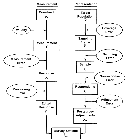
Figure 5.1: Survey life cycle from a quality perspective. Source: Groves et al., 2009, p. 48
Note that this cycle is referred to a single survey statistic and not the whole survey. In practice, the survey designer is expected to minimize all of these sources of errors for particular statistics, but also pay attention to optimizing an overall minimal error in the survey.
5.1 Coverage error
Coverage error refers to a mismatch between the target population and the sampling frame that will actually be used to draw the sample. As mentioned in Section 3.2, it is common for this mismatch to occur, so an important issue is to what extent does or may exist. It can take the form of undercoverage when the sampling frame lacks some units that form part of the target population, e.g., recent employees of the firm that are not in the human resources department outdated list of employees. Also, it may consider overcoverage, when the sampling frame considers units not in the target population, e.g., former employees in the outdated list while our target population refers to actual employees of the firm.
Coverage error is a property of the relation between the sampling frame and the target population for a particular statistic. Thus, it is independent of the drawn sample, as well as it would also affect a census.
The existence of coverage error eventually gives place to coverage bias, i.e., the difference in the statistic due to the mismatch between the sampling frame and the target population. So, let’s imagine that we are interested in the net earnings of employees, specifically, our quantity of interest is the mean of the net earnings of the actual employees of a firm (\(\mu\)). The coverage bias would be defined as:
\[\text{Coverage bias} = \mu_C - \mu\]
Where \(\mu\) is the net earnings’ mean of the target population and \(\mu_C\) is the net earnings’ mean of the units in the sampling frame. Following the example, in Table 5.1 we start with a fictitious sampling frame of 10 people that is outdated:
| Employee | Name | Earnings | Gender |
|---|---|---|---|
| 1 | Noah | 1200 | Male |
| 2 | Ben | 1500 | Male |
| 3 | Paul | 2200 | Male |
| 4 | Leon | 1200 | Male |
| 5 | Luis | 1600 | Male |
| 6 | Emma | 2100 | Female |
| 7 | Mia | 1450 | Female |
| 8 | Emilia | 1500 | Female |
| 9 | Sophia | 1400 | Female |
| 10 | Lina | 1000 | Female |
The mean earnings from the employees in the sampling frame would be (\(\mu_C\)):
But now let’s imagine that we have the data for the actual employees of the firm. Notice that in Table 5.2 there are two employees not in the sampling frame (recently contracted employees) – Jonas and Clara –, leading to undercoverage; as well as two employees in the sampling frame are no longer part of the firm – Luis and Lina –, implying overcoverage.
| Employee | Name | Earnings | Gender |
|---|---|---|---|
| 1 | Noah | 1200 | Male |
| 2 | Ben | 1500 | Male |
| 3 | Paul | 2200 | Male |
| 4 | Leon | 1200 | Male |
| 11 | Jonas | 1300 | Male |
| 6 | Emma | 2100 | Female |
| 7 | Mia | 1450 | Female |
| 8 | Emilia | 1500 | Female |
| 9 | Sophia | 1400 | Female |
| 12 | Clara | 900 | Female |
Now we calculate the mean earnings of the actual employees (\(\mu\)):
In this fictitious example, we confront both undercoverage and overcoverage. We see that if we would rely on the available sampling frame, our quantity of interest would be biased upwards, as the mean earnings of the employees in the sampling frame is higher on average than those in the target population. In particular, in this example we can calculate the coverage bias as:
5.2 Sampling error
Drawing a random sample to represent the population introduces by design a source of error: sampling error. Deliberately leaving out some of the units available on the sampling frame will likely deviate the sample statistic from the same statistic calculated on all of the units on the sampling frame.
There are two types of sampling errors: sampling bias and sampling variance. The former refers to the effect of having units on the sampling frame with no chances (or very low chances) of being selected. This implies that by design in any of the possible samples that could be drawn from the sampling frame these units will be systematically excluded. For example, if in the outdated sampling frame the employee with the highest earnings – Paul – would have a probability of 0 of being selected, the mean earnings for a sample of size 8 will tend to be biased downwards:
sample8 <- sampling_frame %>%
  filter(Name != "Paul") %>% # leave Paul out of the sampling frame
  sample_n(8) # draw a sample of size 8

sample8$Name
#> [1] "Leon"   "Emma"   "Luis"   "Lina"   "Sophia" "Mia"    "Ben"    "Noah"

mean(sample8$Earnings)
#> [1] 1431
In this case the sampling bias is the difference of the mean obtained in the random sample of size 8, 1431, and the mean from the sample frame, 1515. Thus, in this case the sampling bias would be equal to -84, which is a downward bias expected as we deliberately took off the sampling frame the employee with the highest earnings before drawing the random sample.
The sampling variance refers to the variability related to the different possible samples. Although most of the times we only have one sample, it is possible to think and estimate how variable would an estimate be along all of the possible samples. In the case of our sampling frame of 10 employees, given a sample of size 8, we can calculate how many different samples (combinations) of this size can be obtained from such a sampling frame (see also Section 3.1):
\[{10 \choose 8} = \frac{10!}{8!(10-8)!} = 45 \]
The sampling variance refers, then, to how variable the mean earnings would be among these 45 different samples, each of size 8. The distribution of the quantity of interest among all of the possible samples is called sampling distribution. This concept is further developed in Part III.
5.3 Nonresponse error
After a sample is drawn, the fieldwork process begins. A common outcome from this process is that not every sampled unit will actually take part in the survey, for different reasons. In some cases, some units will not be reachable, will not be able to respond or provide information or, when the units are individuals, they might just refuse to participate (see Fig. 3.2). Nonresponse errors arises when there is a difference between the statistic calculated on the actual respondents of the survey and the same statistic for the whole sample. In the example of the firm, we could think that some of the 8 sampled members of Table 5.1 refuse to answer about their earnings for privacy concerns. Given that the quantity of interest is the mean earnings, the nonresponse bias can be expressed similar to the coverage bias:
\[\text{Nonresponse bias} = \bar{x}_{r} - \bar{x}_{s}\]
Where \(\bar{x}_r\) is the mean earnings of the respondents and \(\bar{x}_s\) the mean earnings of the sample.
5.4 Adjustment error
Commonly, postsurvey adjustments are conducted after a survey is conducted. They are aimed at increasing the quality of a sample estimate in the face of coverage, sampling and nonresponse errors. Information about the target population, frame population or response rate of the sample is used to adjust estimates. These adjustments imply weighting the obtained sample data to balance those cases over and underrepresented (by known standards). The adjustment error refers to the difference between an adjusted statistic and the population parameter. So in our example, we know that there is a 50% of men and women in the target population (Table 5.2). A possible sample of size 8 might not have this balance of men and women, as it happens in a new sample of size 8:
sample8 <- sampling_frame %>%
  sample_n(8) # draw a sample of size 8

sample8$Name
#> [1] "Leon"   "Mia"    "Lina"   "Noah"   "Paul"   "Sophia" "Emma"   "Emilia"

mean(sample8$Earnings)
#> [1] 1506
In this case the sample has 5 women (62.5%) and 3 men (37.5%), thus the former are overrepresented and the latter underrepresented. A simple adjustment for calculating mean earnings that can be applied in this case is inverse probability weighting, i.e., to assign a weight to each group so that weighted mean earnings can be obtained with each group having the same weight as in the target population. So, in this case the weight for women would be \(w_i = 1 / 0.625\) and for men \(w_i = 1 / 0.375\).
# Assign weights by group
sample8 <- sample8 %>%
  group_by(Gender) %>%
  mutate(weight = 1 / (n() / 8))

unique(sample8$weight) %>%
  round(2)
#> [1] 2.67 1.60

weighted.mean(x = sample8$Earnings, w = sample8$weight)
#> [1] 1512
The adjustment error in this example could be expressed as:
\[\bar{x}_{adj} - \mu\]
Where \(\bar{x}_{adj}\) is the adjusted mean earnings of the sample (1512) and \(\mu\) the mean of earnings in the population. But as we have assumed that we only have the outdated sampling frame, it would be \(\mu_C\) in this case (1515).
5.5 Other quality criteria
Apart from the measurement and representation dimensions in the total survey error framework, a survey estimate can also be assessed in terms of quality by three other notions:
- Credibility: refers to the judgments done by users regarding the producer of survey estimate. A high credibility is achieved when users judge that the producers have no particular position about the outcomes of the survey. For example, a non-partisan organization that publishes a prediction of an election will tend to have higher credibility than the same prediction published by an organization related to one of the concerned candidates.
- Relevance: a survey estimate is relevant when it measures a construct similar to the requirements of the users. For example, if users are interested in the happiness of individuals, they might only have an indicator of overall life satisfaction which, although closely related, is usually considered as a different construct. In this case, the distance between these constructs makes the available one less relevant.
- Timeliness: making the information available at the needed moment for decisions based on it. This criteria is determined by the use a survey statistic has in practice. For example, if a prediction of an election is published after the actual election takes place it will considerably loose timeliness for most of its users.