3 Ejemplo 2

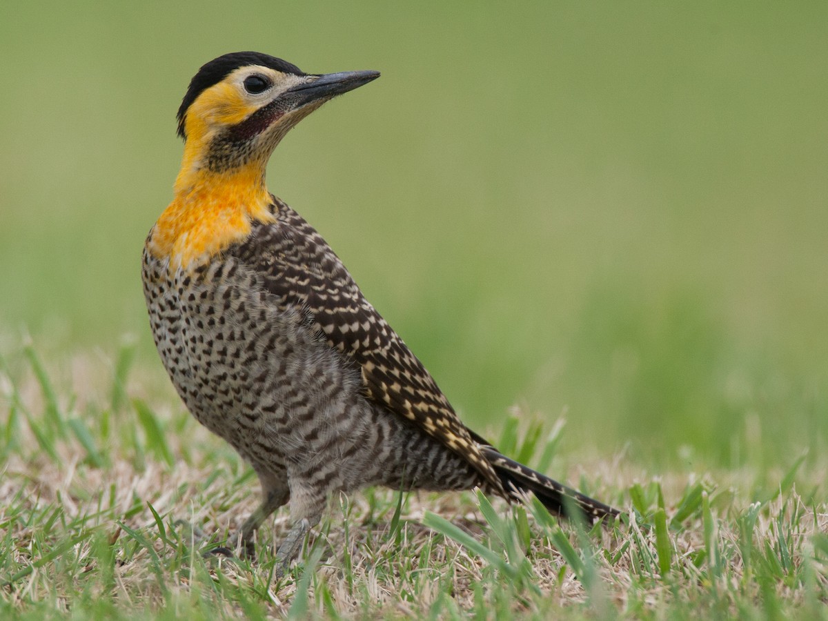
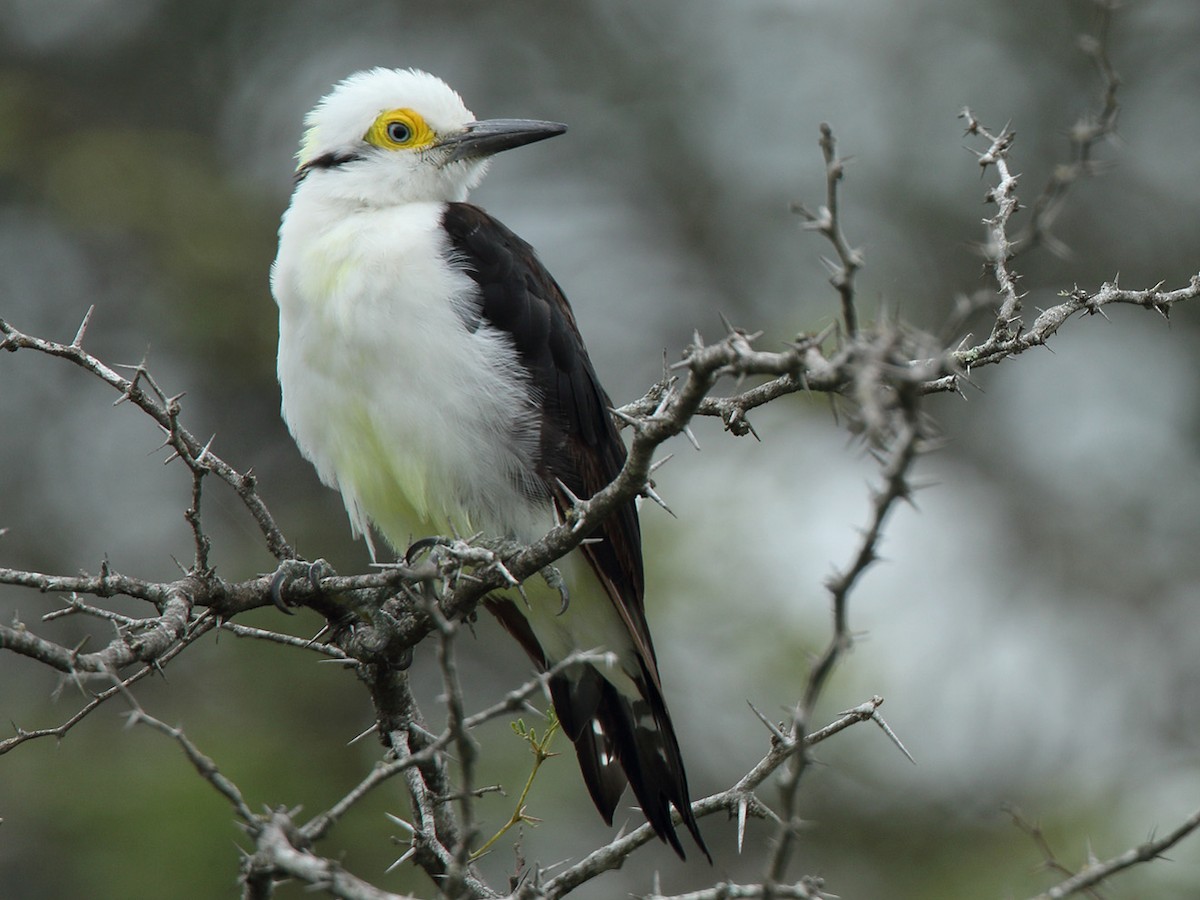
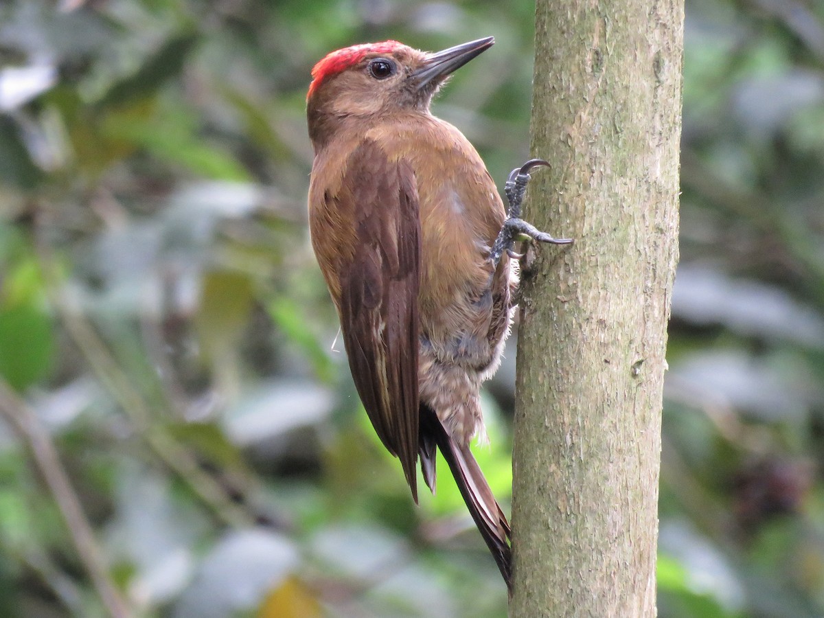
Se realiza un estudio de diversas especies de pájaros que son de similar naturaleza y comparten un medio común. El canto de cada especie tiene un conjunto de rasgos distintivos que permite reconocerla. Una característica investigada es la duración del canto en segundos. Se obtuvieron los siguientes datos:

Colaptes campestris	Melanerpes candidus	Veniliornis fumigatus
1.11	2.17	0.42
1.23	1.85	0.93
0.91	1.99	0.77
0.95	1.74	0.37
0.99	1.54	0.50
1.08	1.86	0.48
1.18	1.87	0.68
1.29	2.04	0.62
1.12	1.69	0.39

Colaptes campestris Melanerpes candidus Veniliornis fumigatus

3.1 LSD

3.1.1 Data.frame

Tratamiento<- factor(rep(c("CC","MC","VF"), each = 9))
Duración<- c(1.11,1.23,0.91,0.95,0.99,1.08,1.18,1.29,1.12,
             2.17,1.85,1.99,1.74,1.54,1.86,1.87,2.04,1.69,
             0.42,0.93,0.77,0.37,0.50,0.48,0.68,0.62,0.39)
datos<- data.frame(Tratamiento,Duración)
head(datos)

##   Tratamiento Duración
## 1          CC     1.11
## 2          CC     1.23
## 3          CC     0.91
## 4          CC     0.95
## 5          CC     0.99
## 6          CC     1.08

str(datos)

## 'data.frame':    27 obs. of  2 variables:
##  $ Tratamiento: Factor w/ 3 levels "CC","MC","VF": 1 1 1 1 1 1 1 1 1 2 ...
##  $ Duración   : num  1.11 1.23 0.91 0.95 0.99 1.08 1.18 1.29 1.12 2.17 ...

3.1.2 ANOVA

ANAVA<- aov(data = datos,Duración~Tratamiento)
summary(ANAVA)

##             Df Sum Sq Mean Sq F value   Pr(>F)    
## Tratamiento  2  7.551   3.776   126.9 1.73e-13 ***
## Residuals   24  0.714   0.030                     
## ---
## Signif. codes:  0 '***' 0.001 '**' 0.01 '*' 0.05 '.' 0.1 ' ' 1

3.1.3 LSD

library(tidyverse)
valor_máximo<-datos %>% 
  group_by(Tratamiento) %>% 
  summarise(máx=max(Duración))
valor_máximo

## # A tibble: 3 × 2
##   Tratamiento   máx
##   <fct>       <dbl>
## 1 CC           1.29
## 2 MC           2.17
## 3 VF           0.93

library(agricolae)

## Warning: package 'agricolae' was built under R version 4.2.3

lsd<- LSD.test(ANAVA, trt = "Tratamiento", group = T)
lsd$means

##     Duración       std r       LCL       UCL  Min  Max  Q25  Q50  Q75
## CC 1.0955556 0.1278780 9 0.9768846 1.2142265 0.91 1.29 0.99 1.11 1.18
## MC 1.8611111 0.1908170 9 1.7424402 1.9797820 1.54 2.17 1.74 1.86 1.99
## VF 0.5733333 0.1910497 9 0.4546624 0.6920043 0.37 0.93 0.42 0.50 0.68

lsd$groups

##     Duración groups
## MC 1.8611111      a
## CC 1.0955556      b
## VF 0.5733333      c

letras_lsd<- lsd$groups[order(row.names(lsd$groups)),]
ggplot(data = datos, aes(x=Tratamiento, y=Duración,fill=Tratamiento))+
  geom_boxplot(show.legend = F)+
  stat_boxplot(geom = "errorbar",width=0.3)+
  geom_text(data = valor_máximo,aes(x = Tratamiento, y = 0.2+ máx,label=letras_lsd$groups, vjust=0))+
  theme_minimal()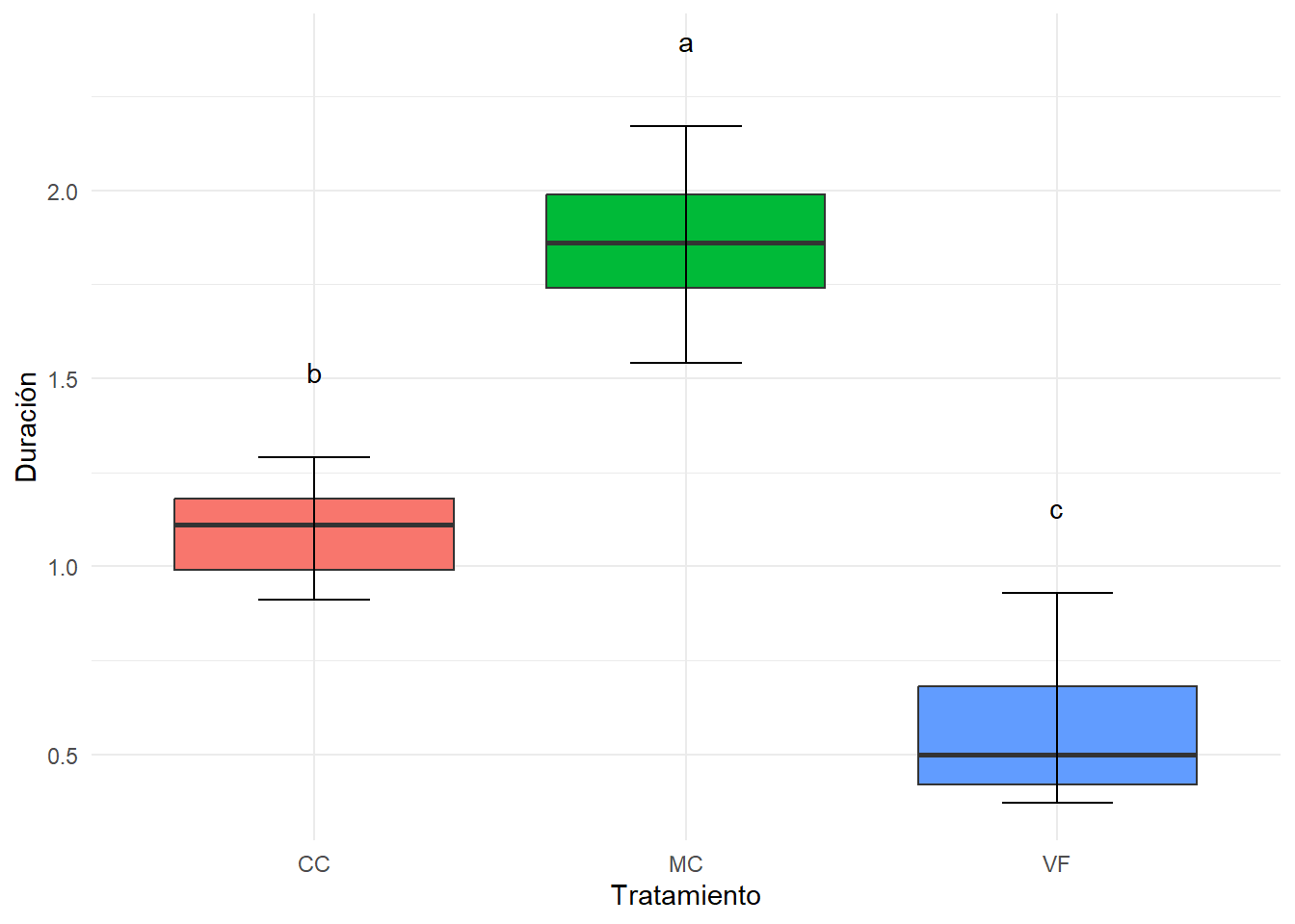

3.2 DUNCAN

Tratamiento<- factor(rep(c("CC","MC","VF"), each = 9))
Duración<- c(1.11,1.23,0.91,0.95,0.99,1.08,1.18,1.29,1.12,
             2.17,1.85,1.99,1.74,1.54,1.86,1.87,2.04,1.69,
             0.42,0.93,0.77,0.37,0.50,0.48,0.68,0.62,0.39)
datos<- data.frame(Tratamiento,Duración)
head(datos)

##   Tratamiento Duración
## 1          CC     1.11
## 2          CC     1.23
## 3          CC     0.91
## 4          CC     0.95
## 5          CC     0.99
## 6          CC     1.08

str(datos)

## 'data.frame':    27 obs. of  2 variables:
##  $ Tratamiento: Factor w/ 3 levels "CC","MC","VF": 1 1 1 1 1 1 1 1 1 2 ...
##  $ Duración   : num  1.11 1.23 0.91 0.95 0.99 1.08 1.18 1.29 1.12 2.17 ...

ANAVA<- aov(data = datos,Duración~Tratamiento)
summary(ANAVA)

##             Df Sum Sq Mean Sq F value   Pr(>F)    
## Tratamiento  2  7.551   3.776   126.9 1.73e-13 ***
## Residuals   24  0.714   0.030                     
## ---
## Signif. codes:  0 '***' 0.001 '**' 0.01 '*' 0.05 '.' 0.1 ' ' 1

library(tidyverse)
valor_máximo<-datos %>% 
  group_by(Tratamiento) %>% 
  summarise(máx=max(Duración))
valor_máximo

## # A tibble: 3 × 2
##   Tratamiento   máx
##   <fct>       <dbl>
## 1 CC           1.29
## 2 MC           2.17
## 3 VF           0.93

library(agricolae)

library(agricolae)
duncan<-duncan.test(ANAVA, trt = "Tratamiento", group = T)
letras_duncan<- duncan$groups[order(row.names(duncan$groups)),]
plot<-ggplot(data = datos, aes(x=Tratamiento, y=Duración,fill=Tratamiento))+
  geom_boxplot(show.legend = F)+
  stat_boxplot(geom = "errorbar",width=0.3)+
  geom_text(data = valor_máximo,aes(x = Tratamiento, y = 0.2+ máx,label=letras_duncan$groups, vjust=0))+
  theme_minimal()
plot + scale_fill_brewer(palette = "Pastel1")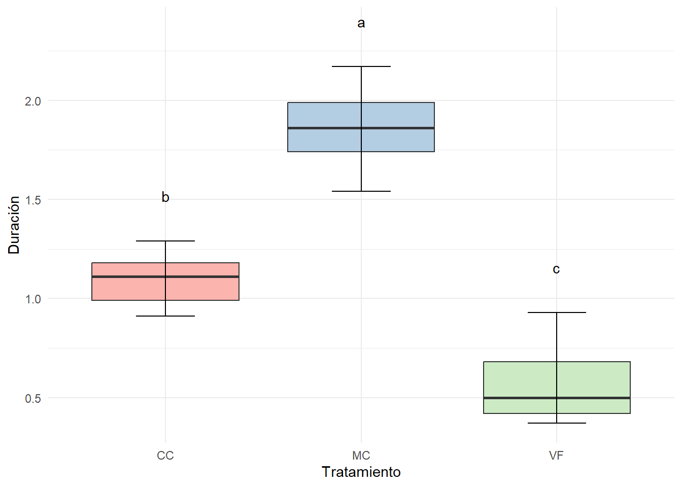

3.3 SCHEFFE

Tratamiento<- factor(rep(c("CC","MC","VF"), each = 9))
Duración<- c(1.11,1.23,0.91,0.95,0.99,1.08,1.18,1.29,1.12,
             2.17,1.85,1.99,1.74,1.54,1.86,1.87,2.04,1.69,
             0.42,0.93,0.77,0.37,0.50,0.48,0.68,0.62,0.39)
datos<- data.frame(Tratamiento,Duración)
head(datos)

##   Tratamiento Duración
## 1          CC     1.11
## 2          CC     1.23
## 3          CC     0.91
## 4          CC     0.95
## 5          CC     0.99
## 6          CC     1.08

str(datos)

## 'data.frame':    27 obs. of  2 variables:
##  $ Tratamiento: Factor w/ 3 levels "CC","MC","VF": 1 1 1 1 1 1 1 1 1 2 ...
##  $ Duración   : num  1.11 1.23 0.91 0.95 0.99 1.08 1.18 1.29 1.12 2.17 ...

ANAVA<- aov(data = datos,Duración~Tratamiento)

scheffe<- scheffe.test(ANAVA, "Tratamiento", group = T, console = T)

## 
## Study: ANAVA ~ "Tratamiento"
## 
## Scheffe Test for Duración 
## 
## Mean Square Error  : 0.02975463 
## 
## Tratamiento,  means
## 
##     Duración       std r  Min  Max
## CC 1.0955556 0.1278780 9 0.91 1.29
## MC 1.8611111 0.1908170 9 1.54 2.17
## VF 0.5733333 0.1910497 9 0.37 0.93
## 
## Alpha: 0.05 ; DF Error: 24 
## Critical Value of F: 3.402826 
## 
## Minimum Significant Difference: 0.2121319 
## 
## Means with the same letter are not significantly different.
## 
##     Duración groups
## MC 1.8611111      a
## CC 1.0955556      b
## VF 0.5733333      c

library(DescTools)

## Warning: package 'DescTools' was built under R version 4.2.3

ScheffeTest(ANAVA)

## 
##   Posthoc multiple comparisons of means: Scheffe Test 
##     95% family-wise confidence level
## 
## $Tratamiento
##             diff     lwr.ci     upr.ci    pval    
## MC-CC  0.7655556  0.5534237  0.9776874 8.8e-09 ***
## VF-CC -0.5222222 -0.7343541 -0.3100904 6.1e-06 ***
## VF-MC -1.2877778 -1.4999096 -1.0756459 2.0e-13 ***
## 
## ---
## Signif. codes:  0 '***' 0.001 '**' 0.01 '*' 0.05 '.' 0.1 ' ' 1