Chapter 8 Exploratory data analysis and feature engineering

8.1 Big data

8.2 But what is it, really?

It’s (kind of) big data when you need:

Distributed processing
Distributed computation
Many machines (clusters)

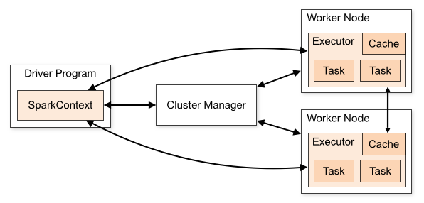
Notes:

Built with inspiration from Google
Open Source
System for distributed processing
Storage: HDFS
Computation - MapReduce, YARN
Splits your data onto different computers
Is used a lot but there are a lot more alternatives these days that outperform hadoop, mainly cloud solutions.
Named after the creator’s sons Elephant toy

8.3 What is it not?

Not for data storage, keep your data somewhere else

8.4 How can we use it in R?

8.5 Now… do you need it?

8.6 The Sparklyr API is really great

You can see all the functions in sparklyr by writing sparklyr:: in R or help(package = "sparklyr").
spark_ for Spark stuff: reading data, configurations etc.
sdf_ Functions for working with Spark DataFrames, ex. sdf_nrow()
ft_ for feature transformers
ml_ for ML functions, pipelines, classifiers
dplyr verbs, most of which can be used on Spark DataFrames

8.7 Set up your Spark context

library(sparklyr)
sc <- spark_connect(master = "local")

## Re-using existing Spark connection to local

sc$config

## $spark.env.SPARK_LOCAL_IP.local
## [1] "127.0.0.1"
## 
## $sparklyr.connect.csv.embedded
## [1] "^1.*"
## 
## $spark.sql.catalogImplementation
## [1] "hive"
## 
## $sparklyr.connect.cores.local
## [1] 4
## 
## $spark.sql.shuffle.partitions.local
## [1] 4
## 
## $`sparklyr.shell.driver-memory`
## [1] "2g"
## 
## attr(,"config")
## [1] "default"
## attr(,"file")
## [1] "/Library/Frameworks/R.framework/Versions/3.6/Resources/library/sparklyr/conf/config-template.yml"

8.8 We can manipulate our configuration

config <- spark_config()

config$`sparklyr.shell.driver-memory` <- "4G"
config$`sparklyr.shell.executor-memory` <- "4G"

sc <- spark_connect(master = "local", config = config)

8.9 Okey, let’s load some data.

Use spark_read_csv() to read the file ml_data into Spark.

spark_read_csv(sc, "ml_data", "/Users/filipwastberg/Documents/ferrologic/r-utbildning-tele2/data/ml_data.csv")

## # Source: spark<ml_data> [?? x 36]
##    ar_key ssn   monthly_data_us… bundle_size avg_monthly_dat…
##    <chr>  <chr>            <dbl> <chr>                  <dbl>
##  1 AAEBf… AAEB…            838   20                    6504. 
##  2 AAEBf… AAEB…            268.  1                      677. 
##  3 AAEBf… AAEB…            233.  1                      576. 
##  4 AAEBf… AAEB…           1105.  5                      828. 
##  5 AAEBf… AAEB…              3.7 5                     2035. 
##  6 AAEBf… AAEB…            721.  5                      741. 
##  7 AAEBf… AAEB…              0   5                      180. 
##  8 AAEBf… AAEB…            565.  5                      585. 
##  9 AAEBf… AAEB…          50457.  9999                 31256. 
## 10 AAEBf… AAEB…             10.7 0.5                     37.4
## # … with more rows, and 31 more variables:
## #   days_till_installment_end <int>, number_of_events <int>,
## #   su_subs_age <int>, cpe_type <chr>, cpe_model <chr>,
## #   cpe_model_days_in_net <int>, cpe_net_type_cmpt <chr>,
## #   pc_priceplan_nm <chr>, days_with_price_plan <int>,
## #   days_with_data_bucket <int>, days_with_contract <int>,
## #   days_since_cstatus_act <int>, current_price_plan <chr>,
## #   count_price_plans <int>, days_since_last_price_plan_change <int>,
## #   days_since_price_plan_launch <int>, hardware_age <int>,
## #   days_since_last_hardware_change <int>, slask_data <int>,
## #   slask_sms <int>, slask_minutes <int>,
## #   weekend_data_usage_by_hour <chr>, weekdays_data_usage_by_hour <chr>,
## #   label <int>, days_till_installment_end_missing <int>,
## #   su_subs_age_missing <int>, cpe_model_days_in_net_missing <int>,
## #   days_since_cstatus_act_missing <int>, days_to_migration_missing <int>,
## #   days_since_last_price_plan_change_missing <int>,
## #   hardware_age_missing <int>

8.10 What’s the plan?

For tele2 data: label indicates that a customer has bought new hardware within 30 days
For telco: churn indicates that a customer has churned

8.11 `sdf_` functions

spark_read_csv(sc, "telco_data", "/Users/filipwastberg/Documents/ferrologic/r-utbildning-tele2/data/telco.csv")

## # Source: spark<telco_data> [?? x 21]
##    customer_id gender senior_citizen partner dependents tenure
##    <chr>       <chr>           <int> <chr>   <chr>       <int>
##  1 7590-VHVEG  Female              0 Yes     No              1
##  2 5575-GNVDE  Male                0 No      No             34
##  3 3668-QPYBK  Male                0 No      No              2
##  4 7795-CFOCW  Male                0 No      No             45
##  5 9237-HQITU  Female              0 No      No              2
##  6 9305-CDSKC  Female              0 No      No              8
##  7 1452-KIOVK  Male                0 No      Yes            22
##  8 6713-OKOMC  Female              0 No      No             10
##  9 7892-POOKP  Female              0 Yes     No             28
## 10 6388-TABGU  Male                0 No      Yes            62
## # … with more rows, and 15 more variables: phone_service <chr>,
## #   multiple_lines <chr>, internet_service <chr>, online_security <chr>,
## #   online_backup <chr>, device_protection <chr>, tech_support <chr>,
## #   streaming_tv <chr>, streaming_movies <chr>, contract <chr>,
## #   paperless_billing <chr>, payment_method <chr>, monthly_charges <dbl>,
## #   total_charges <chr>, churn <chr>

library(dplyr)
telco <- tbl(sc, "telco_data")

sdf_nrow(telco)

## [1] 7043

telco <- telco %>% 
    mutate(total_charges = as.numeric(total_charges))

sdf_dim(telco)

## [1] 7043   21

sdf_describe(telco)

## # Source: spark<?> [?? x 22]
##   summary customer_id gender senior_citizen partner dependents tenure
##   <chr>   <chr>       <chr>  <chr>          <chr>   <chr>      <chr> 
## 1 count   7043        7043   7043           7043    7043       7043  
## 2 mean    <NA>        <NA>   0.16214681243… <NA>    <NA>       32.37…
## 3 stddev  <NA>        <NA>   0.36861160561… <NA>    <NA>       24.55…
## 4 min     0002-ORFBO  Female 0              No      No         0     
## 5 max     9995-HOTOH  Male   1              Yes     Yes        72    
## # … with 15 more variables: phone_service <chr>, multiple_lines <chr>,
## #   internet_service <chr>, online_security <chr>, online_backup <chr>,
## #   device_protection <chr>, tech_support <chr>, streaming_tv <chr>,
## #   streaming_movies <chr>, contract <chr>, paperless_billing <chr>,
## #   payment_method <chr>, monthly_charges <chr>, total_charges <chr>,
## #   churn <chr>

8.12 Exploratory analysis - one of the most important parts

Open a new Rmarkdown-file, use the Spark connection and the sdf_ functions to describe the data-set
How many rows are there?
How many columns?
Any other of the sdf_-functions that you might find useful here?
What type of columns are we dealing with? Use glimpse()

data <- tbl(sc, "ml_data")

sdf_nrow(data)

## [1] 236955

sdf_dim(data)

## [1] 236955     36

sdf_describe(data)

## # Source: spark<?> [?? x 37]
##   summary ar_key ssn   monthly_data_us… bundle_size avg_monthly_dat…
##   <chr>   <chr>  <chr> <chr>            <chr>       <chr>           
## 1 count   236955 2369… 236955           236955      236955          
## 2 mean    <NA>   <NA>  2948.0124487771… 360.530827… 3054.4449912199…
## 3 stddev  <NA>   <NA>  15629.603789775… 1840.45878… 7681.1706544080…
## 4 min     AAEBf… AAEB… 0.0              0.2         4.72526617526618
## 5 max     AAEBf… AAEB… 908605.8         NA          103352.015245082
## # … with 31 more variables: days_till_installment_end <chr>,
## #   number_of_events <chr>, su_subs_age <chr>, cpe_type <chr>,
## #   cpe_model <chr>, cpe_model_days_in_net <chr>, cpe_net_type_cmpt <chr>,
## #   pc_priceplan_nm <chr>, days_with_price_plan <chr>,
## #   days_with_data_bucket <chr>, days_with_contract <chr>,
## #   days_since_cstatus_act <chr>, current_price_plan <chr>,
## #   count_price_plans <chr>, days_since_last_price_plan_change <chr>,
## #   days_since_price_plan_launch <chr>, hardware_age <chr>,
## #   days_since_last_hardware_change <chr>, slask_data <chr>,
## #   slask_sms <chr>, slask_minutes <chr>,
## #   weekend_data_usage_by_hour <chr>, weekdays_data_usage_by_hour <chr>,
## #   label <chr>, days_till_installment_end_missing <chr>,
## #   su_subs_age_missing <chr>, cpe_model_days_in_net_missing <chr>,
## #   days_since_cstatus_act_missing <chr>, days_to_migration_missing <chr>,
## #   days_since_last_price_plan_change_missing <chr>,
## #   hardware_age_missing <chr>

glimpse(data)

## Observations: ??
## Variables: 36
## Database: spark_connection
## $ ar_key                                    <chr> "AAEBfitQf9ubLtKn5vPLq…
## $ ssn                                       <chr> "AAEBfplgfyVbkQtbGKU98…
## $ monthly_data_usage                        <dbl> 838.0, 267.7, 232.8, 1…
## $ bundle_size                               <chr> "20", "1", "1", "5", "…
## $ avg_monthly_data_usage                    <dbl> 6503.50127, 676.96099,…
## $ days_till_installment_end                 <int> NA, NA, NA, 0, NA, NA,…
## $ number_of_events                          <int> 0, 0, 0, 2, 0, 0, 0, 1…
## $ su_subs_age                               <int> 61, 45, 69, 53, 51, 40…
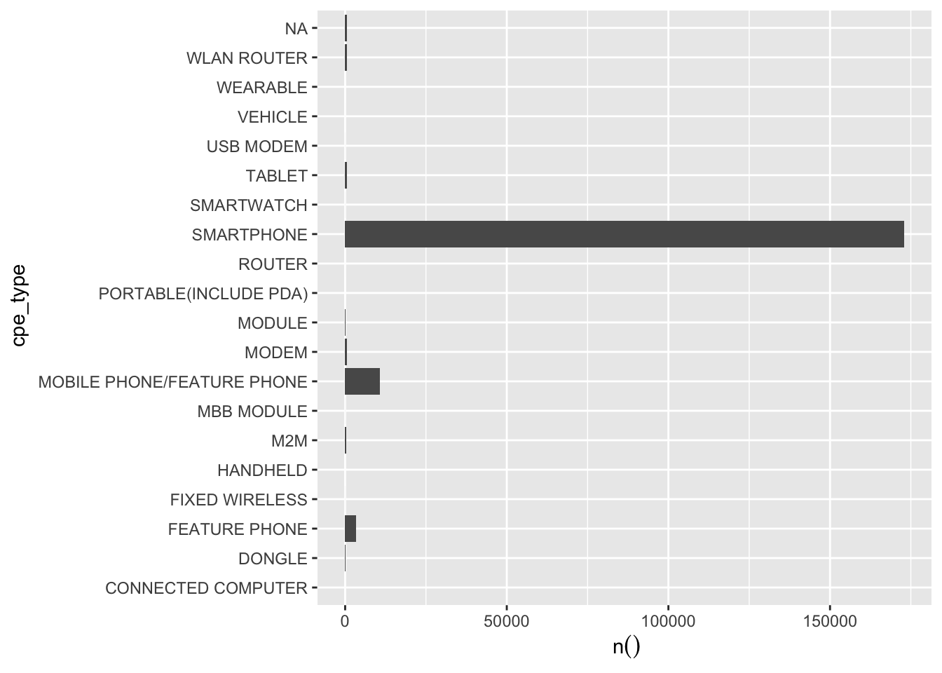
## $ cpe_type                                  <chr> "SMARTPHONE", "SMARTPH…
## $ cpe_model                                 <chr> "SAMSUNG SM-A520F", "S…
## $ cpe_model_days_in_net                     <int> 687, 670, 970, 1223, 2…
## $ cpe_net_type_cmpt                         <chr> "4G", "4G", "3.5G", "4…
## $ pc_priceplan_nm                           <chr> "Fast pris", "Fast pri…
## $ days_with_price_plan                      <int> 1039, 623, 619, 580, 8…
## $ days_with_data_bucket                     <int> 1039, 623, 619, 580, 8…
## $ days_with_contract                        <int> 4793, 2258, 3618, 3393…
## $ days_since_cstatus_act                    <int> 4792, 2257, 3617, 3392…
## $ current_price_plan                        <chr> "Fast pris", "Fast pri…
## $ count_price_plans                         <int> 1, 1, 1, 1, 1, 1, 1, 1…
## $ days_since_last_price_plan_change         <int> NA, NA, NA, NA, NA, NA…
## $ days_since_price_plan_launch              <int> 509, 514, 509, 465, 51…
## $ hardware_age                              <int> NA, NA, 970, 1223, 205…
## $ days_since_last_hardware_change           <int> 509, 449, 428, 465, 51…
## $ slask_data                                <int> 0, 0, 0, 0, 0, 0, 1, 0…
## $ slask_sms                                 <int> 0, 0, 0, 0, 0, 0, 0, 0…
## $ slask_minutes                             <int> 0, 0, 0, 0, 1, 0, 0, 0…
## $ weekend_data_usage_by_hour                <chr> "569188|506524|598717|…
## $ weekdays_data_usage_by_hour               <chr> "2031595|1308209|14445…
## $ label                                     <int> 0, 0, 0, 0, 0, 0, 0, 0…
## $ days_till_installment_end_missing         <int> 1, 1, 1, 0, 1, 1, 0, 0…
## $ su_subs_age_missing                       <int> 0, 0, 0, 0, 0, 0, 0, 0…
## $ cpe_model_days_in_net_missing             <int> 0, 0, 0, 0, 0, 0, 0, 0…
## $ days_since_cstatus_act_missing            <int> 0, 0, 0, 0, 0, 0, 0, 0…
## $ days_to_migration_missing                 <int> 1, 1, 1, 1, 1, 1, 1, 1…
## $ days_since_last_price_plan_change_missing <int> 1, 1, 1, 1, 1, 1, 1, 1…
## $ hardware_age_missing                      <int> 1, 1, 0, 0, 0, 0, 0, 0…

8.13 Distribution of NA’s

We can easily calculate how many NA’s there are in one variable.

telco %>% 
  filter(is.na(gender)) %>% 
  sdf_nrow()

## [1] 0

8.14 If we want to do it for all variables

Map over all columns

library(purrr)
sdf_count_na <- function(tbl){
    df <-   map_df(set_names(colnames(tbl)), function(x){
        sym_x <- sym(x) ## Convert from string to variable name
        count <- tbl %>% 
            filter(is.na({{sym_x}})) %>% 
            sdf_nrow() 
        
        perc = count / sdf_nrow(tbl)
        
        tibble::tibble(variable = x,
                       count_na = count,
                       perc_na = perc)
    })
    return(df)
}

sdf_count_na(telco)

## # A tibble: 21 x 3
##    variable         count_na perc_na
##    <chr>               <dbl>   <dbl>
##  1 customer_id             0       0
##  2 gender                  0       0
##  3 senior_citizen          0       0
##  4 partner                 0       0
##  5 dependents              0       0
##  6 tenure                  0       0
##  7 phone_service           0       0
##  8 multiple_lines          0       0
##  9 internet_service        0       0
## 10 online_security         0       0
## # … with 11 more rows

8.14.1 Excercise

Using the function sdf_count_na() and plot the NA’s in data.

8.15 EDA

Exploratory data analysis is a crucial part of modelling
We check the data quality
Try to understand relationships between variables
Do some initial feature selection

8.16 Split the data

Split the data into a training data set and a test data set
Do it before we do EDA
The test data should always be left untouched, we are building a model for future data

split <- sdf_random_split(telco, training = 0.8, testing = 0.2, seed = 123)
telco_train <- split$training
telco_test <- split$testing

8.17 Continue in your Rmarkdown-file

Split your data into a training and a test data set
Do some exploratory analysis on the training data with dplyr and ggplot2
How are the variables distributed?
When looking on non numeric columns, reflect how we should represent these columns
What is the balance of our the column label that we will model?
Are there some variables that you can exclude right away?

8.18 Check out the correlations

ml_corr() returns a correlation matrix
Can only be performed on numeric variables
Cannot calculate on columns where NA is present

corrs <- telco_train %>% 
    mutate(churn = if_else(churn == "Yes", 1, 0)) %>% 
    select_if(is.numeric) %>% 
    filter_all(all_vars(!is.na(.))) %>% 
    ml_corr(method = "spearman")

## Applying predicate on the first 100 rows

corrs

## # A tibble: 5 x 5
##   senior_citizen   tenure monthly_charges total_charges  churn
##            <dbl>    <dbl>           <dbl>         <dbl>  <dbl>
## 1        1        0.00166           0.220        0.0893  0.157
## 2        0.00166  1                 0.248        0.826  -0.355
## 3        0.220    0.248             1            0.652   0.191
## 4        0.0893   0.826             0.652        1      -0.200
## 5        0.157   -0.355             0.191       -0.200   1

library(corrplot)

## corrplot 0.84 loaded

rownames(corrs) <- colnames(corrs)

## Warning: Setting row names on a tibble is deprecated.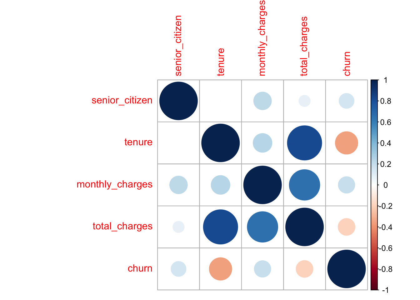

p <- corrplot(as.matrix(corrs))

##                 senior_citizen       tenure monthly_charges total_charges
## senior_citizen     1.000000000  0.001661928       0.2201380    0.08934403
## tenure             0.001661928  1.000000000       0.2482641    0.82568781
## monthly_charges    0.220138022  0.248264057       1.0000000    0.65193752
## total_charges      0.089344030  0.825687814       0.6519375    1.00000000
## churn              0.157315884 -0.354637331       0.1912939   -0.19984998
##                      churn
## senior_citizen   0.1573159
## tenure          -0.3546373
## monthly_charges  0.1912939
## total_charges   -0.1998500
## churn            1.0000000

8.18.1 Excercise

Select data without the columns with more than 5% NA
Select all numeric columns
Filter out NA’s in all columns
Perform a correlation
Plot the correlations using corrplot

split <- sdf_random_split(data, training = 0.8, testing = 0.2, seed = 123)
data_train <- split$training
data_test <- split$testing

corr <- data_train %>% 
    select(-days_till_installment_end,
                                -hardware_age,
                                -days_since_last_price_plan_change,
                                -contains("missing"),
                                -contains("slask")) %>% 
    select_if(is.numeric) %>% 
    filter_all(all_vars(!is.na(.))) %>% 
    ml_corr()

## Applying predicate on the first 100 rows

rownames(corr) <- colnames(corr)

## Warning: Setting row names on a tibble is deprecated.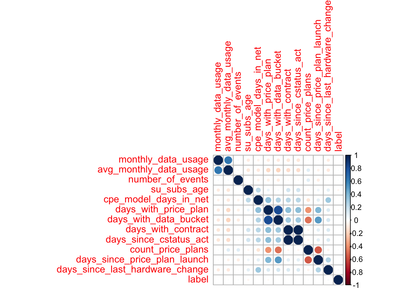

p <- corrplot(as.matrix(corr))

##                                 monthly_data_usage avg_monthly_data_usage
## monthly_data_usage                     1.000000000             0.63837369
## avg_monthly_data_usage                 0.638373695             1.00000000
## number_of_events                       0.021815578             0.02752415
## su_subs_age                           -0.084111289            -0.10940726
## cpe_model_days_in_net                 -0.050737917            -0.09789949
## days_with_price_plan                  -0.085475722            -0.16690347
## days_with_data_bucket                 -0.090544693            -0.18363272
## days_with_contract                    -0.107778831            -0.14801766
## days_since_cstatus_act                -0.106970697            -0.14685774
## count_price_plans                      0.019855345             0.10724979
## days_since_price_plan_launch          -0.011175298            -0.05654132
## days_since_last_hardware_change       -0.080613402            -0.09795793
## label                                  0.007520593             0.01009601
##                                 number_of_events  su_subs_age
## monthly_data_usage                   0.021815578 -0.084111289
## avg_monthly_data_usage               0.027524153 -0.109407257
## number_of_events                     1.000000000  0.005081406
## su_subs_age                          0.005081406  1.000000000
## cpe_model_days_in_net               -0.053775790  0.227542381
## days_with_price_plan                -0.069796317  0.061589769
## days_with_data_bucket               -0.080225104  0.026668894
## days_with_contract                  -0.021402259  0.158323019
## days_since_cstatus_act              -0.020098086  0.158541650
## count_price_plans                    0.107591305 -0.038170407
## days_since_price_plan_launch        -0.078408700  0.056349805
## days_since_last_hardware_change     -0.012082386  0.094563318
## label                                0.016624310 -0.031919701
##                                 cpe_model_days_in_net days_with_price_plan
## monthly_data_usage                       -0.050737917          -0.08547572
## avg_monthly_data_usage                   -0.097899492          -0.16690347
## number_of_events                         -0.053775790          -0.06979632
## su_subs_age                               0.227542381           0.06158977
## cpe_model_days_in_net                     1.000000000           0.35712772
## days_with_price_plan                      0.357127719           1.00000000
## days_with_data_bucket                     0.253539171           0.81068435
## days_with_contract                        0.236099081           0.36557152
## days_since_cstatus_act                    0.233369638           0.36115841
## count_price_plans                        -0.115841577          -0.39499206
## days_since_price_plan_launch              0.096388013           0.39389175
## days_since_last_hardware_change           0.316724794           0.12016943
## label                                    -0.006194509          -0.02109536
##                                 days_with_data_bucket days_with_contract
## monthly_data_usage                       -0.090544693       -0.107778831
## avg_monthly_data_usage                   -0.183632723       -0.148017660
## number_of_events                         -0.080225104       -0.021402259
## su_subs_age                               0.026668894        0.158323019
## cpe_model_days_in_net                     0.253539171        0.236099081
## days_with_price_plan                      0.810684349        0.365571518
## days_with_data_bucket                     1.000000000        0.304215352
## days_with_contract                        0.304215352        1.000000000
## days_since_cstatus_act                    0.300879436        0.991821224
## count_price_plans                        -0.484626285       -0.039901414
## days_since_price_plan_launch              0.505118662        0.099445782
## days_since_last_hardware_change           0.141507799        0.121451941
## label                                    -0.009593701       -0.009780062
##                                 days_since_cstatus_act count_price_plans
## monthly_data_usage                        -0.106970697        0.01985535
## avg_monthly_data_usage                    -0.146857737        0.10724979
## number_of_events                          -0.020098086        0.10759130
## su_subs_age                                0.158541650       -0.03817041
## cpe_model_days_in_net                      0.233369638       -0.11584158
## days_with_price_plan                       0.361158408       -0.39499206
## days_with_data_bucket                      0.300879436       -0.48462628
## days_with_contract                         0.991821224       -0.03990141
## days_since_cstatus_act                     1.000000000       -0.03906575
## count_price_plans                         -0.039065746        1.00000000
## days_since_price_plan_launch               0.097950300       -0.55497863
## days_since_last_hardware_change            0.120532322       -0.04983192
## label                                     -0.009201517        0.01134957
##                                 days_since_price_plan_launch
## monthly_data_usage                              -0.011175298
## avg_monthly_data_usage                          -0.056541325
## number_of_events                                -0.078408700
## su_subs_age                                      0.056349805
## cpe_model_days_in_net                            0.096388013
## days_with_price_plan                             0.393891749
## days_with_data_bucket                            0.505118662
## days_with_contract                               0.099445782
## days_since_cstatus_act                           0.097950300
## count_price_plans                               -0.554978626
## days_since_price_plan_launch                     1.000000000
## days_since_last_hardware_change                  0.258665510
## label                                           -0.004290405
##                                 days_since_last_hardware_change
## monthly_data_usage                                  -0.08061340
## avg_monthly_data_usage                              -0.09795793
## number_of_events                                    -0.01208239
## su_subs_age                                          0.09456332
## cpe_model_days_in_net                                0.31672479
## days_with_price_plan                                 0.12016943
## days_with_data_bucket                                0.14150780
## days_with_contract                                   0.12145194
## days_since_cstatus_act                               0.12053232
## count_price_plans                                   -0.04983192
## days_since_price_plan_launch                         0.25866551
## days_since_last_hardware_change                      1.00000000
## label                                                0.02728020
##                                        label
## monthly_data_usage               0.007520593
## avg_monthly_data_usage           0.010096006
## number_of_events                 0.016624310
## su_subs_age                     -0.031919701
## cpe_model_days_in_net           -0.006194509
## days_with_price_plan            -0.021095355
## days_with_data_bucket           -0.009593701
## days_with_contract              -0.009780062
## days_since_cstatus_act          -0.009201517
## count_price_plans                0.011349569
## days_since_price_plan_launch    -0.004290405
## days_since_last_hardware_change  0.027280204
## label                            1.000000000

8.19 Ideally we want to calculate the probability that a customer will buy new hardware within 30 days

We know that the response is not normally distributed, thus there can be no linear relationship between input and output variables
We know that a lot of columns are not normally distributed
We suspect that some columns are highly dependent

In other words: there is a lot to do in terms of feature engineering

8.20 Feature engineering

8.21 What is feature engineering?

The process of creating representations of data that increase the effectiveness of a model.
The goal with feature engineering may differ - what is effectiveness?
A complex model may not be the best model even if accuracy is higher
Example: suppose we are to hire a newly graduated data analyst
Another example: suppose we are to buy a house or apartment and we know every school’s quality. How do we represent this?
Different models are sensitive to different things
Some models work poorly when predictors measure the same underlying
Most models cannot use samples with missing values
Some models may work poorly if irrelevant predictors are included

8.22 Some terminology that surely isn’t new to you

Overfitting
Supervised and unsupervised models
The “No Free Lunch” theorem
Variance vs bias tradeoff
Data driven vs experience driven

8.23 Sparklyr basics reminder

spark_ for Spark stuff: reading data, configurations etc.
sdf_ Functions for working with Spark DataFrames, ex. sdf_nrow()
ft_ for feature transformers <<
ml_ for ML functions, pipelines, classifiers
dplyr verbs, most of which can be used on Spark DataFrames

8.24 There are generally two ways that we can do feature engineering with sparklyr.

As feature transformers with ft_-functions
Or with dplyr (SQL-transformations)

8.24.1 ExcerciseBut first let’s clean our data set a bit

Remove the columns with more than 50% missing values
Remove the corresponding columns that indicate missing values
Make use of select() and combine with the help function contains()
Save your data-set with sdf_register()

data_train <- data_train %>% 
    select(-days_till_installment_end,
                                -days_since_last_price_plan_change,
                                -contains("missing"),
                                -ar_key,
                                -ssn)

data_train %>% 
    head()

## # Source: spark<?> [?? x 25]
##   monthly_data_us… bundle_size avg_monthly_dat… number_of_events
##              <dbl> <chr>                  <dbl>            <int>
## 1          32769.  9999                  85776.                0
## 2           2141.  15                     1902.               92
## 3           7586.  8                      1937.                1
## 4              2.9 1                       576.                0
## 5            148.  5                       828.                0
## 6             33.8 3                      2833.                0
## # … with 21 more variables: su_subs_age <int>, cpe_type <chr>,
## #   cpe_model <chr>, cpe_model_days_in_net <int>, cpe_net_type_cmpt <chr>,
## #   pc_priceplan_nm <chr>, days_with_price_plan <int>,
## #   days_with_data_bucket <int>, days_with_contract <int>,
## #   days_since_cstatus_act <int>, current_price_plan <chr>,
## #   count_price_plans <int>, days_since_price_plan_launch <int>,
## #   hardware_age <int>, days_since_last_hardware_change <int>,
## #   slask_data <int>, slask_sms <int>, slask_minutes <int>,
## #   weekend_data_usage_by_hour <chr>, weekdays_data_usage_by_hour <chr>,
## #   label <int>

8.25 Feature transformers

There are lot’s of different feature transformers for feature engineering

Imputations
String indexing
String manipulation such as tokenization, hashing etc.
Scaling/normalizing
Binning continuoues variables to categories
And more…

8.26 Imputations

How do we replace missing values?
ft_imputer(input_cols, output_cols, strategy = "mean")
Mean or median

input_cols <- c("total_charges")
output_cols <- paste0(input_cols, "_imp")

telco_train <- telco_train %>% 
    ft_imputer(input_cols = input_cols, output_cols = output_cols, strategy = "mean")

8.27 How do we impute missing values for categorical variables?

Any ideas?

8.28 Excerices

Create imputations for your numerical columns that has missing values, what strategy do you use?
Make sure you mutate_at() them to be numerical before using ft_imputer()

input_cols <- c("su_subs_age", "hardware_age", "days_since_cstatus_act", "cpe_model_days_in_net")
output_cols <- paste0(input_cols, "_imp")

data_train <- data_train %>% 
    mutate_at(vars(input_cols), as.numeric) %>% 
    ft_imputer(input_cols = input_cols, output_cols = output_cols, strategy = "median")

sdf_count_na(data_train)

## # A tibble: 29 x 3
##    variable               count_na  perc_na
##    <chr>                     <dbl>    <dbl>
##  1 monthly_data_usage            0 0       
##  2 bundle_size                   0 0       
##  3 avg_monthly_data_usage        0 0       
##  4 number_of_events              0 0       
##  5 su_subs_age                  79 0.000416
##  6 cpe_type                    575 0.00303 
##  7 cpe_model                   175 0.000922
##  8 cpe_model_days_in_net       863 0.00455 
##  9 cpe_net_type_cmpt          3091 0.0163  
## 10 pc_priceplan_nm               0 0       
## # … with 19 more rows

8.29 How to handle categories

Dummy variables or one hot encoding
Dummy variables are created when you run a model

telco_train %>% 
    select(-customer_id) %>% 
    filter_all(all_vars(!is.na(.))) %>% 
    ml_logistic_regression(churn ~ .)

## Formula: churn ~ .
## 
## Coefficients:
##                              (Intercept) 
##                            -1.5386100263 
##                            gender_Female 
##                             0.0826419074 
##                           senior_citizen 
##                             0.1878384333 
##                               partner_No 
##                            -0.0056405447 
##                            dependents_No 
##                             0.2261885628 
##                                   tenure 
##                            -0.0629009464 
##                        phone_service_Yes 
##                             0.0708491735 
##                        multiple_lines_No 
##                            -0.2052677875 
##                       multiple_lines_Yes 
##                             0.2349775363 
##             internet_service_Fiber optic 
##                             1.0848003244 
##                     internet_service_DSL 
##                            -0.3968966089 
##                       online_security_No 
##                             0.5097397872 
##                      online_security_Yes 
##                             0.2482698691 
##                         online_backup_No 
##                             0.3949884255 
##                        online_backup_Yes 
##                             0.3591913570 
##                     device_protection_No 
##                             0.3322126613 
##                    device_protection_Yes 
##                             0.4278876415 
##                          tech_support_No 
##                             0.5097214542 
##                         tech_support_Yes 
##                             0.2481167988 
##                          streaming_tv_No 
##                             0.1430657372 
##                         streaming_tv_Yes 
##                             0.6099709328 
##                      streaming_movies_No 
##                             0.1187710844 
##                     streaming_movies_Yes 
##                             0.6351014596 
##                  contract_Month-to-month 
##                             0.7370993683 
##                        contract_Two year 
##                            -0.5123167717 
##                    paperless_billing_Yes 
##                             0.3141614316 
##          payment_method_Electronic check 
##                             0.3234089441 
##              payment_method_Mailed check 
##                            -0.0263000024 
## payment_method_Bank transfer (automatic) 
##                             0.0718597067 
##                          monthly_charges 
##                            -0.0309630423 
##                            total_charges 
##                             0.0001766649 
##                        total_charges_imp 
##                             0.0001766649

8.30 Makes sense with data that is evenly distributed

library(ggplot2)
p <- telco_train %>% 
    group_by(payment_method) %>% 
    count() %>% 
    ggplot(aes(x = payment_method, y = n)) + 
    geom_col() +
    coord_flip()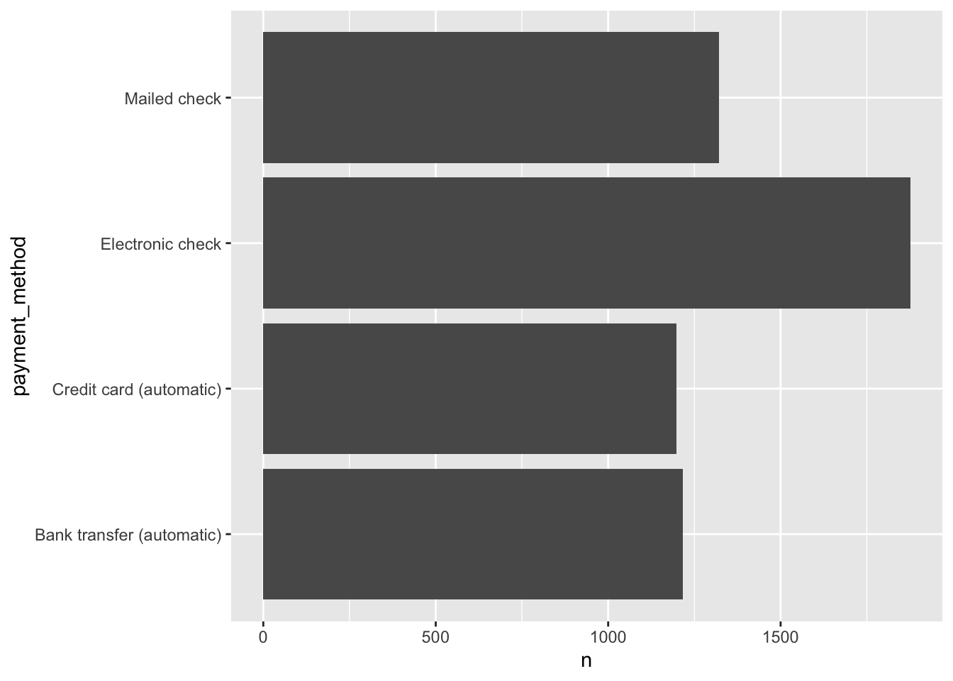

8.31 You can use `ft_string_indexer` and `ft_one_hot_encoder_estimator` to create them manually

telco_train %>% 
    ft_string_indexer(input_col = "payment_method", output_col = "payment_method_i") %>% 
    ft_one_hot_encoder_estimator(input_col = "payment_method_i", output_col = "payment_method_oh") %>% 
    select(-customer_id, -payment_method, -payment_method_i, -total_charges) %>% 
    ml_logistic_regression(churn ~ .)

## Formula: churn ~ .
## 
## Coefficients:
##                                 (Intercept) 
##                                -1.603118097 
##                               gender_Female 
##                                 0.082987267 
##                              senior_citizen 
##                                 0.184810716 
##                                  partner_No 
##                                -0.001895329 
##                               dependents_No 
##                                 0.235572876 
##                                      tenure 
##                                -0.060119785 
##                           phone_service_Yes 
##                                 0.083850527 
##                           multiple_lines_No 
##                                -0.201981904 
##                          multiple_lines_Yes 
##                                 0.236281969 
##                internet_service_Fiber optic 
##                                 1.092155726 
##                        internet_service_DSL 
##                                -0.399614620 
##                          online_security_No 
##                                 0.511871755 
##                         online_security_Yes 
##                                 0.250793359 
##                            online_backup_No 
##                                 0.397095604 
##                           online_backup_Yes 
##                                 0.361723256 
##                        device_protection_No 
##                                 0.334111082 
##                       device_protection_Yes 
##                                 0.430620204 
##                             tech_support_No 
##                                 0.510528075 
##                            tech_support_Yes 
##                                 0.252259533 
##                             streaming_tv_No 
##                                 0.144565189 
##                            streaming_tv_Yes 
##                                 0.613036501 
##                         streaming_movies_No 
##                                 0.116703866 
##                        streaming_movies_Yes 
##                                 0.642089075 
##                     contract_Month-to-month 
##                                 0.747204224 
##                           contract_Two year 
##                                -0.552806498 
##                       paperless_billing_Yes 
##                                 0.313090837 
##                             monthly_charges 
##                                -0.030860312 
##                           total_charges_imp 
##                                 0.000326014 
##          payment_method_oh_Electronic check 
##                                 0.324207797 
##              payment_method_oh_Mailed check 
##                                -0.024251998 
## payment_method_oh_Bank transfer (automatic) 
##                                 0.069876058

8.32 But what about when they are not evenly distributed?

library(ggplot2)
p <- dbplot::dbplot_bar(data_train, cpe_type) +
    coord_flip()

To include all these categories may cause trouble
There’s a risk some cateogry may be in test data but not in train data and vice versa
One way to solve this is by simply creating one dummy for the largest one

8.32.1 Excercise

Take a look at you categorical variables, if you would use them in a model? How would you categorize them?
Feature engineer your categorical variables

8.33 But what if you have a large number of categories?

cpe_models <- data_train %>% 
    group_by(cpe_model) %>% 
    count(sort = T)

cpe_models <- data_train %>% 
    group_by(cpe_model) %>% 
    count(sort = T) %>% 
    filter(n < 20) %>% 
    collect() %>% 
    .$cpe_model

data_train <- data_train %>% 
    mutate(cpe_model_new = if_else(cpe_model %in% cpe_models, "Other", cpe_model))

But to use this in a model might be inefficient

8.34 Feature hashing

A technique common in database querys
A way to store many categories and reduce them by using a hash function

data_train %>% 
    ft_feature_hasher(input_col = "cpe_model_new", output_col = "cpe_model_hash", num_features = 100) %>% 
    select(cpe_model_new, cpe_model_hash) %>% 
    head()

## # Source: spark<?> [?? x 2]
##   cpe_model_new           cpe_model_hash
##   <chr>                   <list>        
## 1 HUAWEI B525S-23A        <dbl [100]>   
## 2 APPLE IPHONE 6S (A1688) <dbl [100]>   
## 3 APPLE IPHONE 6S (A1688) <dbl [100]>   
## 4 NOKIA 206.1             <dbl [100]>   
## 5 APPLE IPHONE 8 (A1905)  <dbl [100]>   
## 6 APPLE IPHONE 6 (A1586)  <dbl [100]>

8.35 A word of caution

What are we trying to capture in the cpe_model is the property of phone type
Are there other variables that more precisely capture what we’re looking for?
Sometimes feature engineering may be asking for more data

8.36 Numerical transformations

Trick question - what distribution is this?

p <- telco_train %>% 
    dbplot::dbplot_histogram(total_charges)

## Warning: Removed 1 rows containing missing values (position_stack).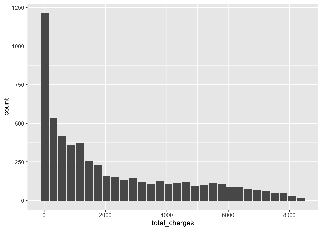

set.seed(2019)
df <- tibble(nb = rnbinom(10000, mu = 500, size = 0.5))

p <- ggplot(df, aes(x = nb)) +
    geom_histogram()

## `stat_bin()` using `bins = 30`. Pick better value with `binwidth`.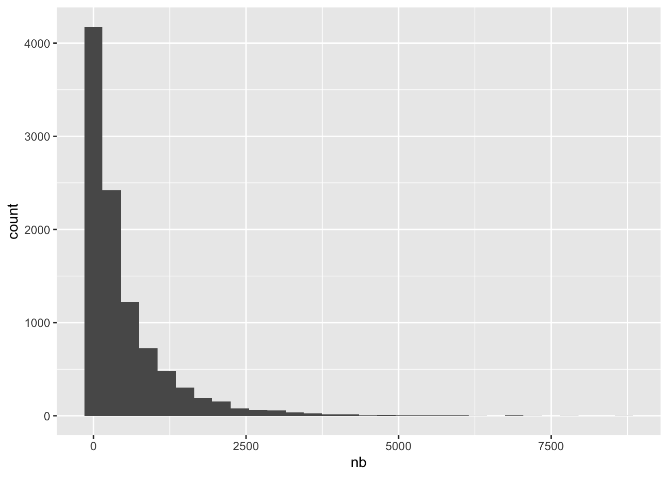

p <- df %>% 
    mutate(fr = log(asin(sqrt(nb / (max(nb) + 1))) + asin(sqrt((nb + 1) / (max(nb) + 1))))) %>% 
    ggplot(aes(x = fr)) +
    geom_density()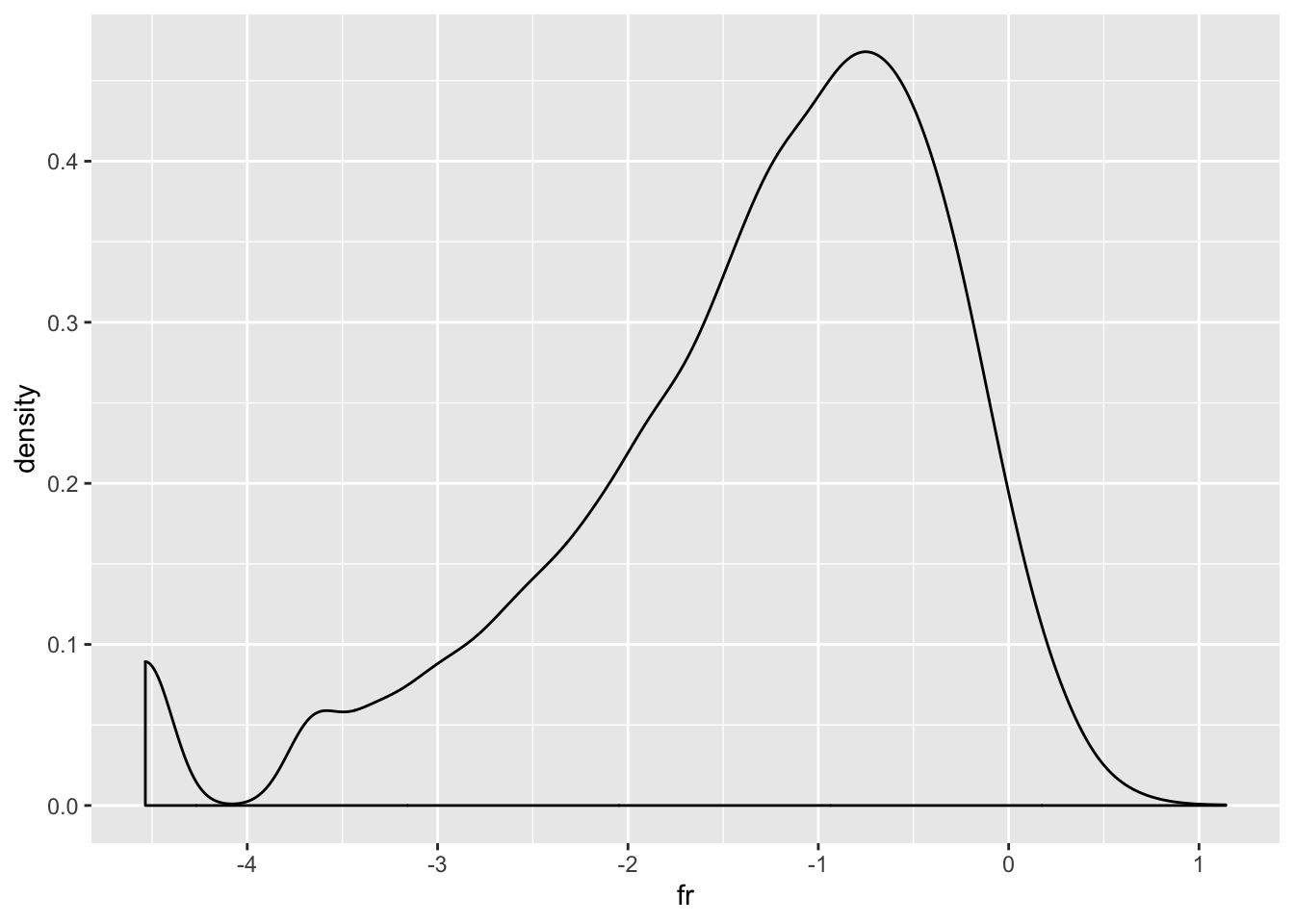

telco_train %>% 
    mutate(log_total_charges = log(total_charges + 1)) %>% 
    dbplot::dbplot_histogram(log_total_charges)

## Warning: Removed 1 rows containing missing values (position_stack).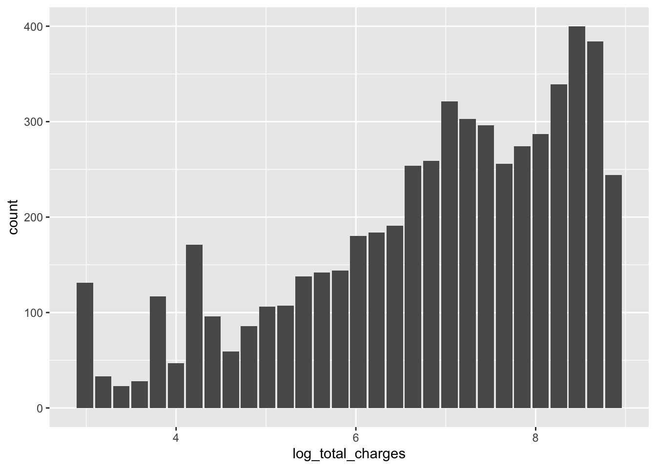

telco_train %>% 
    mutate(log_total_charges = log(asin(sqrt(total_charges / (max(total_charges) + 1))) + 
                                                                                                                                    asin(sqrt((total_charges + 1) / (max(total_charges) + 1))))) %>% 
    dbplot::dbplot_histogram(log_total_charges)

## Warning: Missing values are always removed in SQL.
## Use `MAX(x, na.rm = TRUE)` to silence this warning
## This warning is displayed only once per session.

## Warning: Removed 1 rows containing missing values (position_stack).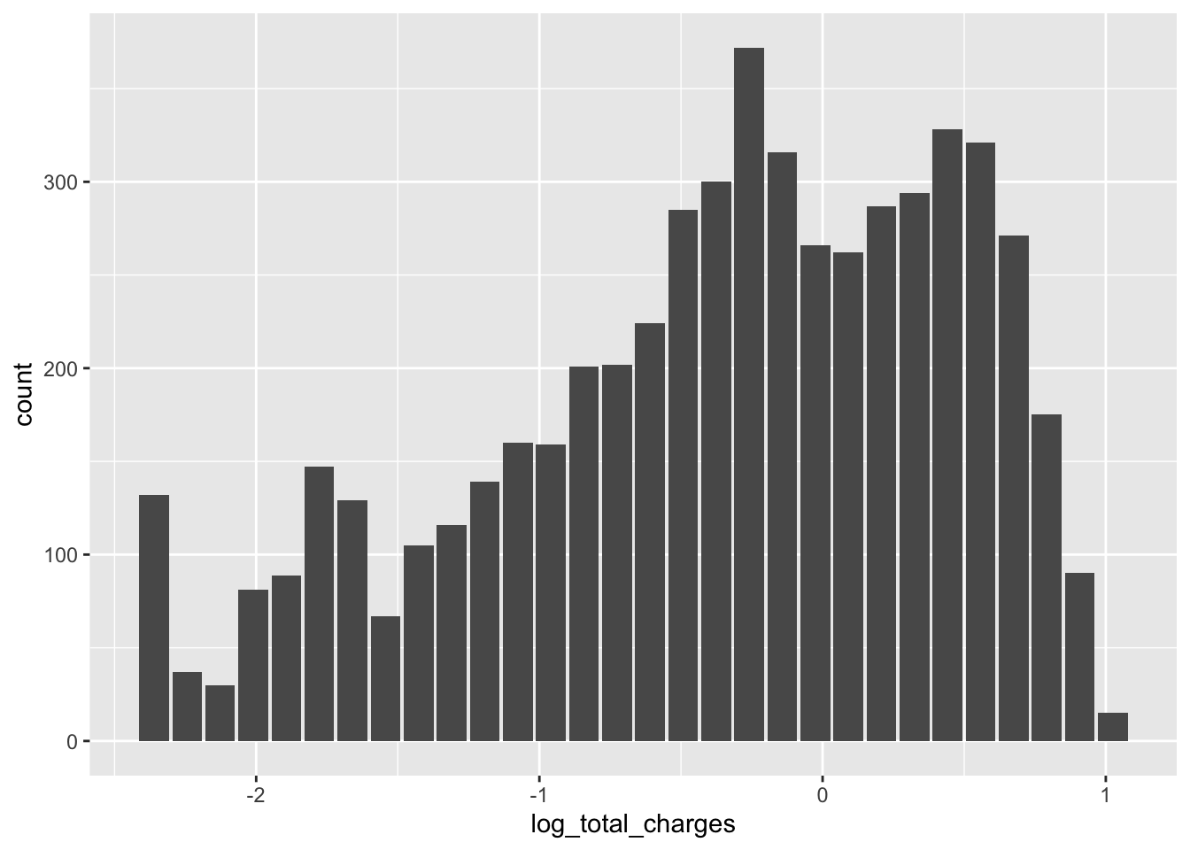

8.36.1 Excercise

Take a look at the numerical columns in your EDA, can you think of a suitable transformation of them?
Transform the columns you think should be transformed

8.37 Rescaling

ft_standard_scaler()
ft_min_max_scaler()
ft_max_abs_scaler()
ft_normalizer()

8.38 Rescaling can improve some models

But it is in unsupervised techniques such as kmeans and principal componant analysis where it’s most important

8.39 Before applying a scale function you need to assemble your vector

telco_train %>% 
    ft_vector_assembler(input_col = c("total_charges_imp", "monthly_charges"), output_col = "charges_temp") %>% 
    ft_standard_scaler(input_col = "charges_temp", output_col = "charges_scaled") %>% 
    select(total_charges_imp, monthly_charges, charges_scaled) %>% 
    head()

## # Source: spark<?> [?? x 3]
##   total_charges_imp monthly_charges charges_scaled
##               <dbl>           <dbl> <list>        
## 1              593.            65.6 <dbl [2]>     
## 2              267.            83.9 <dbl [2]>     
## 3              571.            69.4 <dbl [2]>     
## 4             7904.           110.  <dbl [2]>     
## 5             5378.            84.6 <dbl [2]>     
## 6             5958.            90.4 <dbl [2]>

8.40 You can also scale with dplyr

scaled <- telco_train %>% 
    summarise(max_charges = max(total_charges_imp),
                                        min_charges = min(total_charges_imp)) %>% 
    collect()

## Warning: Missing values are always removed in SQL.
## Use `MAX(x, na.rm = TRUE)` to silence this warning
## This warning is displayed only once per session.

## Warning: Missing values are always removed in SQL.
## Use `MIN(x, na.rm = TRUE)` to silence this warning
## This warning is displayed only once per session.

telco_train <- telco_train %>% 
    mutate(tot_charges_scaled = (total_charges_imp - !!scaled$min_charges) / (!!scaled$max_charges - !!scaled$min_charges))

p <- dbplot::dbplot_histogram(telco_train, tot_charges_scaled)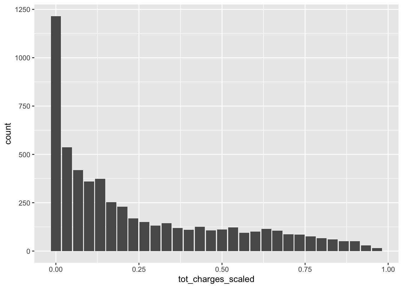

8.40.1 Excercise

Scale some of your columns using on of the scale functions

input_assemble <- c("monthly_data_usage", "avg_monthly_data_usage", 
                                                                                "cpe_model_days_in_net_imp", "days_with_price_plan",
                                                                                "days_with_data_bucket", "hardware_age_imp",
                                                                                "days_since_price_plan_launch")

data_train %>% 
    ft_vector_assembler(input_col = input_assemble, output_col = "ft") %>% 
    ft_min_max_scaler(input_col = "ft", output_col = "ft_scaled") %>% 
    head()

## # Source: spark<?> [?? x 32]
##   monthly_data_us… bundle_size avg_monthly_dat… number_of_events
##              <dbl> <chr>                  <dbl>            <int>
## 1          32769.  9999                  85776.                0
## 2           2141.  15                     1902.               92
## 3           7586.  8                      1937.                1
## 4              2.9 1                       576.                0
## 5            148.  5                       828.                0
## 6             33.8 3                      2833.                0
## # … with 28 more variables: su_subs_age <dbl>, cpe_type <chr>,
## #   cpe_model <chr>, cpe_model_days_in_net <dbl>, cpe_net_type_cmpt <chr>,
## #   pc_priceplan_nm <chr>, days_with_price_plan <int>,
## #   days_with_data_bucket <int>, days_with_contract <int>,
## #   days_since_cstatus_act <dbl>, current_price_plan <chr>,
## #   count_price_plans <int>, days_since_price_plan_launch <int>,
## #   hardware_age <dbl>, days_since_last_hardware_change <int>,
## #   slask_data <int>, slask_sms <int>, slask_minutes <int>,
## #   weekend_data_usage_by_hour <chr>, weekdays_data_usage_by_hour <chr>,
## #   label <int>, su_subs_age_imp <dbl>, hardware_age_imp <dbl>,
## #   days_since_cstatus_act_imp <dbl>, cpe_model_days_in_net_imp <dbl>,
## #   cpe_model_new <chr>, ft <list>, ft_scaled <list>

8.41 Bucketizing

Create categories out of numerical data.
ft_bucketizer let’s you create categories where you define your splits.
Can be useful when a continuoues column doesn’t make sense, for example with age.

telco_train %>% 
    ft_bucketizer(input_col = "tenure", output_col = "tenure_bucket", splits = c(-Inf, 10, 30, 50, Inf)) %>% 
    select(tenure, tenure_bucket) %>% 
    head()

## # Source: spark<?> [?? x 2]
##   tenure tenure_bucket
##    <int>         <dbl>
## 1      9             0
## 2      3             0
## 3      9             0
## 4     71             3
## 5     63             3
## 6     65             3

telco_train %>% 
ft_quantile_discretizer(input_col = "tenure", output_col = "tenure_bucket", num_buckets = 5) %>% 
    select(tenure, tenure_bucket) %>% 
    head()

## # Source: spark<?> [?? x 2]
##   tenure tenure_bucket
##    <int>         <dbl>
## 1      9             1
## 2      3             0
## 3      9             1
## 4     71             4
## 5     63             4
## 6     65             4

8.41.1 Excercise

Which of your numeric variables would make sense to bucketize?
Bucketize at least one of your numerical variables - which strategy do you use?

8.42 Dimensionality reduction

The curse of dimentionality
Principal component analysis
Kmeans clustering or other clustering algorithms.

8.43 PCA

p <- telco_train %>% 
    select(total_charges_imp, monthly_charges) %>% 
    dbplot::dbplot_raster(monthly_charges, total_charges_imp)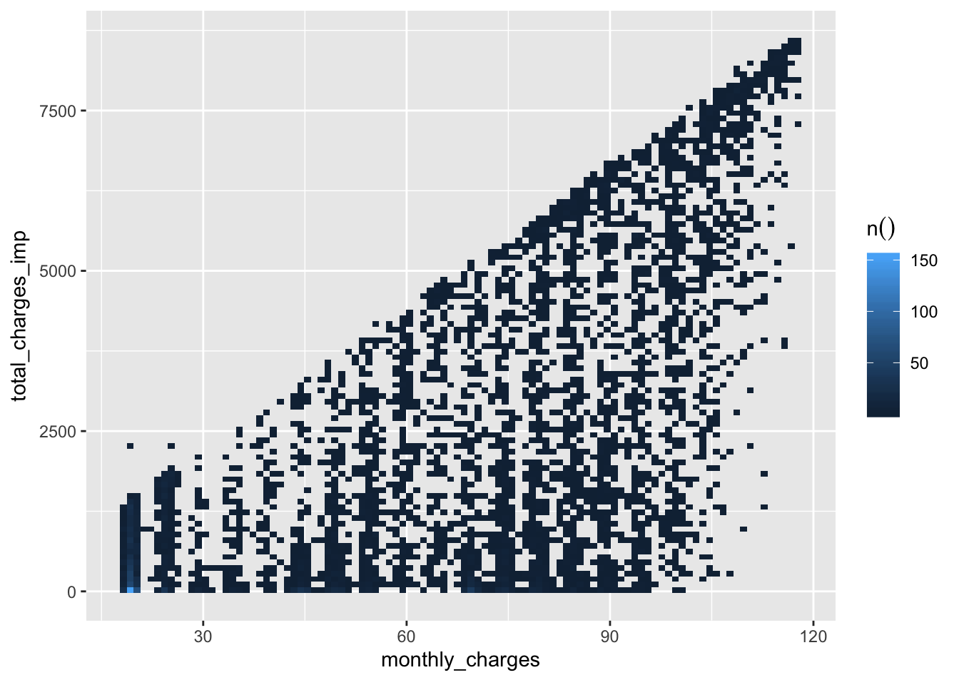

telco_train %>% 
    select(total_charges_imp, monthly_charges) %>% 
    ft_vector_assembler(input_cols = c("total_charges_imp", "monthly_charges"), output_col = "charges_as") %>% 
    ft_standard_scaler(input_col = "charges_as", output_col = "charges_scaled") %>% 
    ft_pca(input_col = "charges_scaled", output_col = "charges_pca", k = 2) %>% 
    ft_pca(input_col = "charges_scaled", output_col = "charges_pca_one", k = 1) %>% 
    head()

## # Source: spark<?> [?? x 6]
##   total_charges_i… monthly_charges charges_as charges_scaled charges_pca
##              <dbl>           <dbl> <list>     <list>         <list>     
## 1             593.            65.6 <dbl [2]>  <dbl [2]>      <dbl [2]>  
## 2             267.            83.9 <dbl [2]>  <dbl [2]>      <dbl [2]>  
## 3             571.            69.4 <dbl [2]>  <dbl [2]>      <dbl [2]>  
## 4            7904.           110.  <dbl [2]>  <dbl [2]>      <dbl [2]>  
## 5            5378.            84.6 <dbl [2]>  <dbl [2]>      <dbl [2]>  
## 6            5958.            90.4 <dbl [2]>  <dbl [2]>      <dbl [2]>  
## # … with 1 more variable: charges_pca_one <list>

8.44 Interactions

interact_sneak <- telco_train %>% 
    select(total_charges_imp, monthly_charges) %>% 
    ft_interaction(input_cols = c("total_charges_imp", "monthly_charges"), output_col = "charges_interact") %>% 
    head() %>% 
    collect()

8.44.1 sdf_register()

When you are done with your feature engineering you can save your new features to a separate spark data.frame

telco_train_fe <- telco_train %>% 
    select(total_charges_imp, monthly_charges) %>% 
    ft_interaction(input_cols = c("total_charges_imp", "monthly_charges"), output_col = "charges_interact") %>% 
    sdf_register("teclot_train_fe")

8.45 Last excercise

Gather all your feature engineering into one script
Perform them and register them as a new spark data.frame

8.46 Modelling with sparklyr

Sparklyr focues on machine learning/predicitve modelling rather than statistical inference
Supports a wide range of ML-algorithms
Is an API to the Apache Spark MLib (there are also great API’s for Scala and Python)
We will focus on functionality rather than specific algorithms

8.47 `ml_` functions

You have seen them during the workshop

library(sparklyr)
library(tidyverse)
sc <- spark_connect(master = "local")

## Re-using existing Spark connection to local

spark_read_csv(sc, "telco_data", "/Users/filipwastberg/Documents/ferrologic/r-utbildning-tele2/data/telco.csv")

## # Source: spark<telco_data> [?? x 21]
##    customer_id gender senior_citizen partner dependents tenure
##    <chr>       <chr>           <int> <chr>   <chr>       <int>
##  1 7590-VHVEG  Female              0 Yes     No              1
##  2 5575-GNVDE  Male                0 No      No             34
##  3 3668-QPYBK  Male                0 No      No              2
##  4 7795-CFOCW  Male                0 No      No             45
##  5 9237-HQITU  Female              0 No      No              2
##  6 9305-CDSKC  Female              0 No      No              8
##  7 1452-KIOVK  Male                0 No      Yes            22
##  8 6713-OKOMC  Female              0 No      No             10
##  9 7892-POOKP  Female              0 Yes     No             28
## 10 6388-TABGU  Male                0 No      Yes            62
## # … with more rows, and 15 more variables: phone_service <chr>,
## #   multiple_lines <chr>, internet_service <chr>, online_security <chr>,
## #   online_backup <chr>, device_protection <chr>, tech_support <chr>,
## #   streaming_tv <chr>, streaming_movies <chr>, contract <chr>,
## #   paperless_billing <chr>, payment_method <chr>, monthly_charges <dbl>,
## #   total_charges <chr>, churn <chr>

telco <- tbl(sc, "telco_data") %>% 
    mutate(total_charges = as.numeric(total_charges))

split <- sdf_random_split(telco, training = 0.8, testing = 0.2, seed = 123)
telco_train <- split$training
telco_test <- split$testing

8.48 The feature engineering is done

telco_train <- telco_train %>% 
    ft_imputer(input_cols = "total_charges", output_cols = "total_charges_imp", strategy = "mean") %>% 
    ft_vector_assembler(input_cols = c("total_charges_imp", "monthly_charges"), output_col = "charges_as") %>% 
    mutate(
        total_charges_log = log(total_charges_imp),
        monthly_charges_log = log(monthly_charges)
    ) %>% 
    select(-customer_id)

8.49 Fitting models

Using the ml_ functions fitting a model is easy
Take a moment just to glance through the list of models available by typing ml_

8.50 Fitting a logistic regression

glr <- ml_logistic_regression(
    telco_train,
    churn ~ total_charges_log + monthly_charges_log + senior_citizen + partner + 
        tenure + phone_service + multiple_lines + internet_service + online_security +
        online_backup + device_protection + tech_support + streaming_tv +
        streaming_movies + contract + paperless_billing + payment_method
    )

8.51 Evaluating the model

eval_glr <- ml_evaluate(glr, telco_train)

eval_glr$area_under_roc()

## [1] 0.8544172

eval_glr <- ml_evaluate(glr, telco_train)

eval_glr$accuracy()

## [1] 0.8080556

eval_glr$false_positive_rate_by_label()

## [1] 0.46014735 0.09470617

eval_glr$recall_by_threshold()

## # Source: spark<?> [?? x 2]
##    threshold recall
##        <dbl>  <dbl>
##  1     0.942 0.0328
##  2     0.866 0.0643
##  3     0.843 0.104 
##  4     0.811 0.136 
##  5     0.789 0.165 
##  6     0.764 0.195 
##  7     0.745 0.217 
##  8     0.730 0.244 
##  9     0.705 0.267 
## 10     0.688 0.291 
## # … with more rows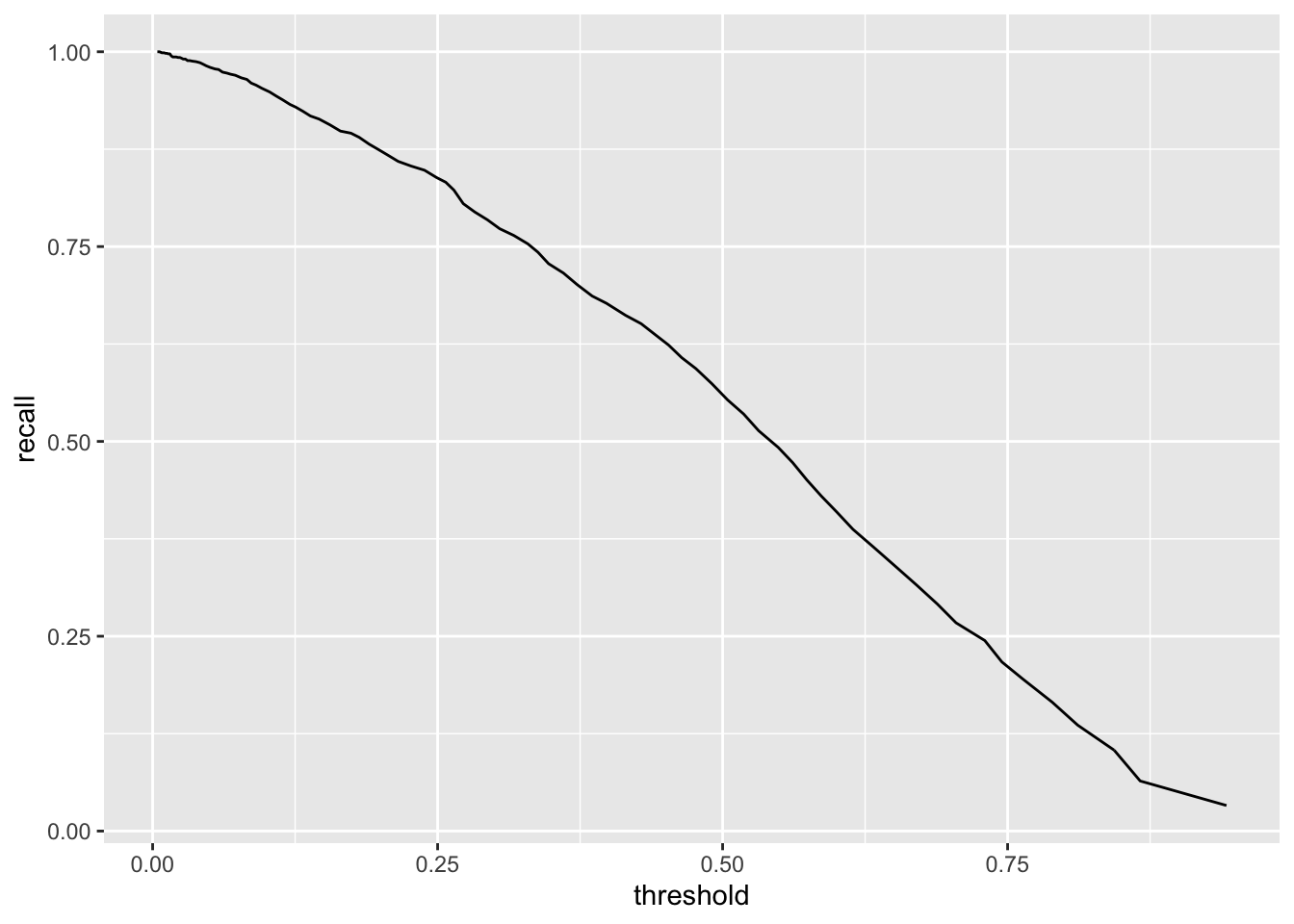

p <- eval_glr$recall_by_threshold() %>% 
    ggplot(aes(threshold, recall)) +
    geom_line()

eval <- ml_evaluate(glr, telco_train)

p <- eval$roc() %>% 
collect() %>% 
    ggplot(aes(FPR, TPR)) +
    geom_line()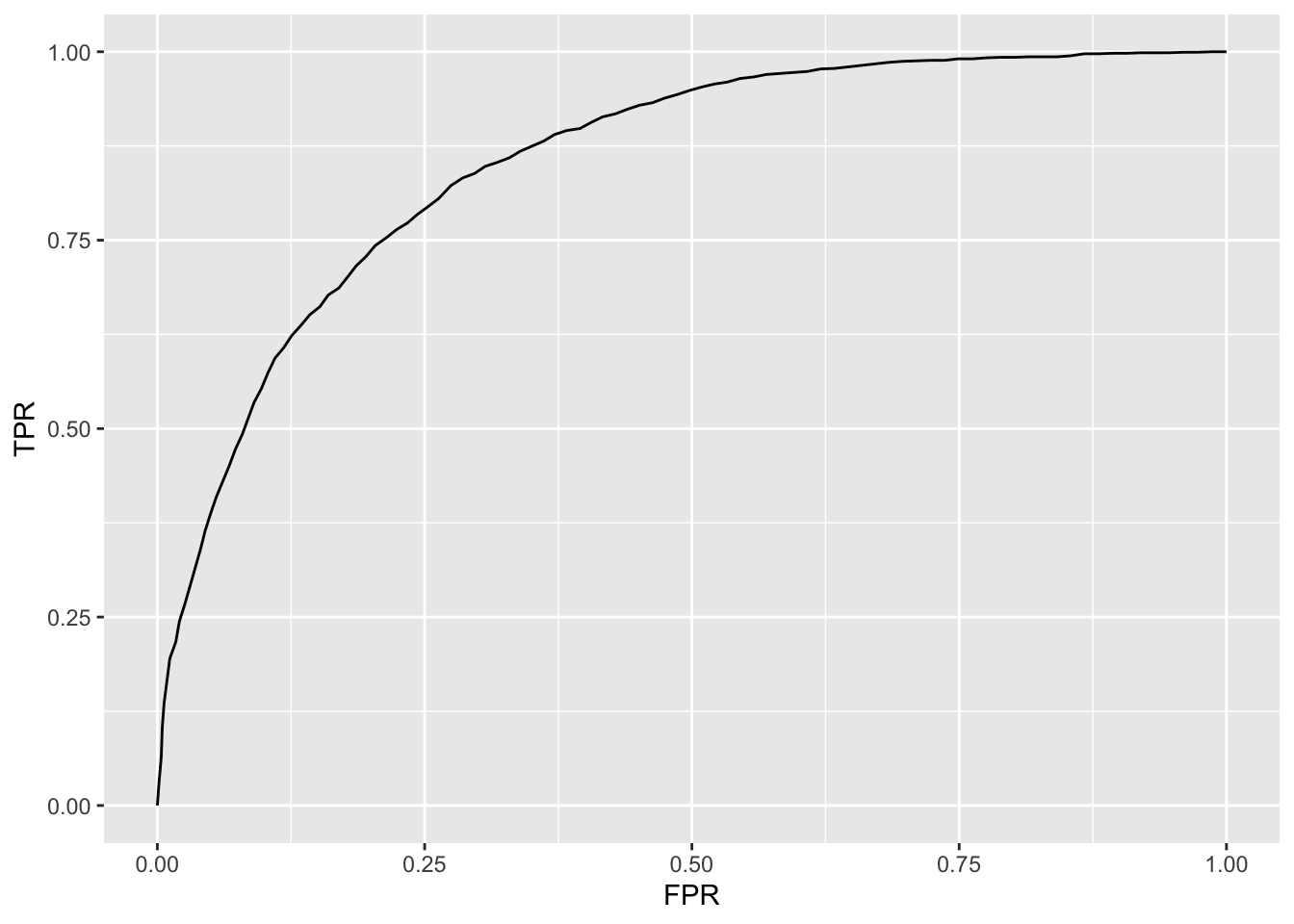

8.51.1 Excercise

Fit a logistic regression on your training data set
Which columns do include/exclude? Keep in mind your EDA
What kind of accuracy measurement do you use?
Plot roc and recall

spark_read_csv(sc, "ml_data", "/Users/filipwastberg/Documents/ferrologic/r-utbildning-tele2/data/ml_data.csv")

## # Source: spark<ml_data> [?? x 36]
##    ar_key ssn   monthly_data_us… bundle_size avg_monthly_dat…
##    <chr>  <chr>            <dbl> <chr>                  <dbl>
##  1 AAEBf… AAEB…            838   20                    6504. 
##  2 AAEBf… AAEB…            268.  1                      677. 
##  3 AAEBf… AAEB…            233.  1                      576. 
##  4 AAEBf… AAEB…           1105.  5                      828. 
##  5 AAEBf… AAEB…              3.7 5                     2035. 
##  6 AAEBf… AAEB…            721.  5                      741. 
##  7 AAEBf… AAEB…              0   5                      180. 
##  8 AAEBf… AAEB…            565.  5                      585. 
##  9 AAEBf… AAEB…          50457.  9999                 31256. 
## 10 AAEBf… AAEB…             10.7 0.5                     37.4
## # … with more rows, and 31 more variables:
## #   days_till_installment_end <int>, number_of_events <int>,
## #   su_subs_age <int>, cpe_type <chr>, cpe_model <chr>,
## #   cpe_model_days_in_net <int>, cpe_net_type_cmpt <chr>,
## #   pc_priceplan_nm <chr>, days_with_price_plan <int>,
## #   days_with_data_bucket <int>, days_with_contract <int>,
## #   days_since_cstatus_act <int>, current_price_plan <chr>,
## #   count_price_plans <int>, days_since_last_price_plan_change <int>,
## #   days_since_price_plan_launch <int>, hardware_age <int>,
## #   days_since_last_hardware_change <int>, slask_data <int>,
## #   slask_sms <int>, slask_minutes <int>,
## #   weekend_data_usage_by_hour <chr>, weekdays_data_usage_by_hour <chr>,
## #   label <int>, days_till_installment_end_missing <int>,
## #   su_subs_age_missing <int>, cpe_model_days_in_net_missing <int>,
## #   days_since_cstatus_act_missing <int>, days_to_migration_missing <int>,
## #   days_since_last_price_plan_change_missing <int>,
## #   hardware_age_missing <int>

data <- tbl(sc, "ml_data")

split <- sdf_random_split(data, training = 0.8, testing = 0.2, seed = 123)

data_train <- split$training
data_test <- split$testing

input_cols <- c("su_subs_age", "hardware_age", "days_since_cstatus_act", "cpe_model_days_in_net")
output_cols <- paste0(input_cols, "_imp")

data_train_scaled <- data_train %>% 
    mutate_at(vars(input_cols), as.numeric) %>% 
    ft_imputer(input_cols = input_cols, output_cols = output_cols, strategy = "median") %>% 
    ft_vector_assembler(input_cols = c("avg_monthly_data_usage", "number_of_events",
                                                                                                                                                "days_with_price_plan", "days_with_contract",
                                                                                                                                                "days_since_price_plan_launch", 
                                                                                                                                                "hardware_age_imp", "cpe_model_days_in_net_imp"),
                                                                                    output_col = "ft_to_scale") %>% 
    ft_standard_scaler(input_col = "ft_to_scale", output_col = "ft_scaled") %>% 
    ft_quantile_discretizer(input_col = "su_subs_age_imp",
                                                                                                    output_col = "age_quant", num_buckets = 5) %>% 
    ft_one_hot_encoder(input_col = "age_quant", output_col = "age_quant_oh")  ## one hot encode for dummy creation

glr_t2 <-   ml_logistic_regression(data_train_scaled, label ~ ft_scaled + age_quant)
    
eval <- ml_evaluate(glr_t2, data_train_scaled)

eval$area_under_roc()

## [1] 0.611234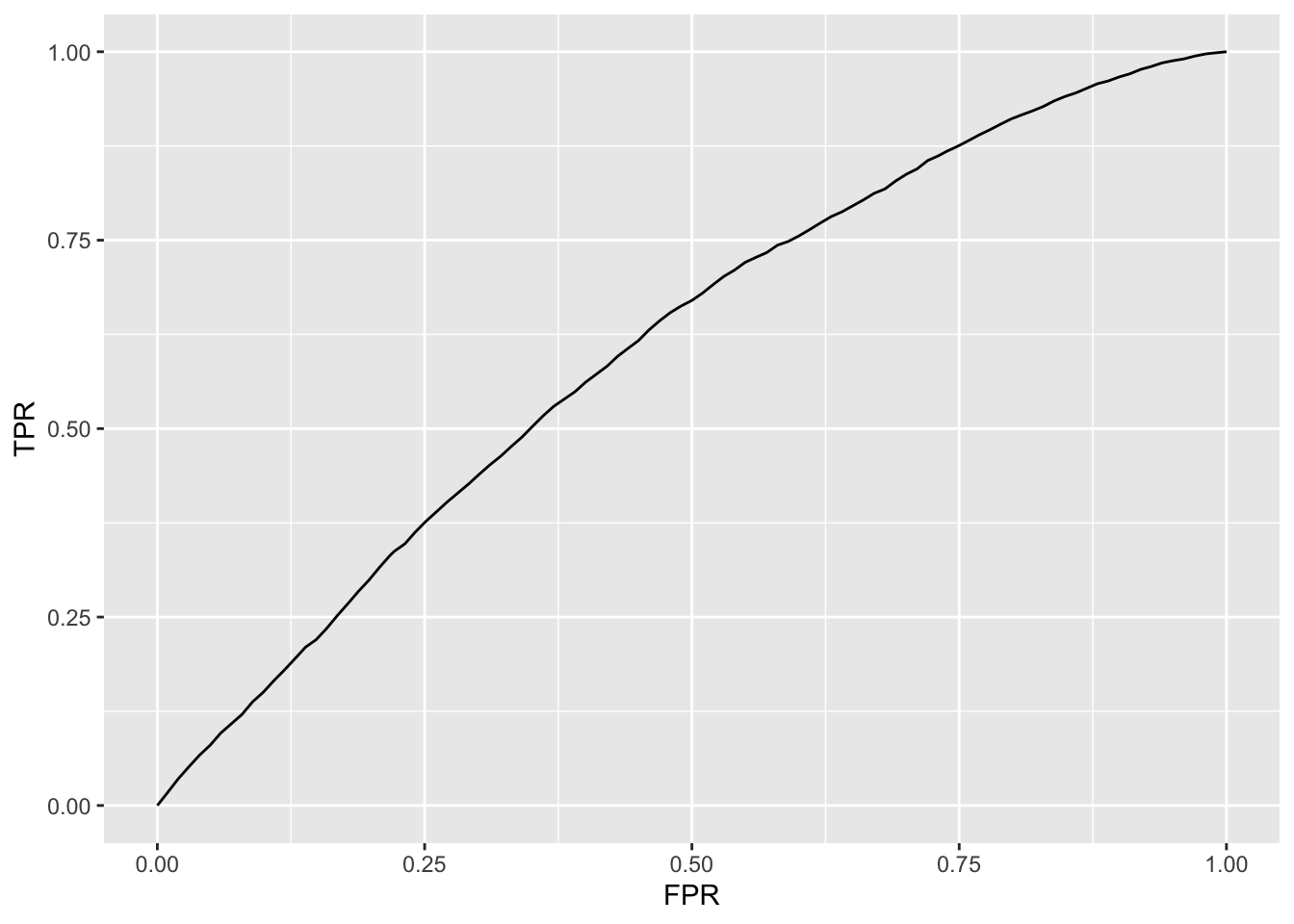

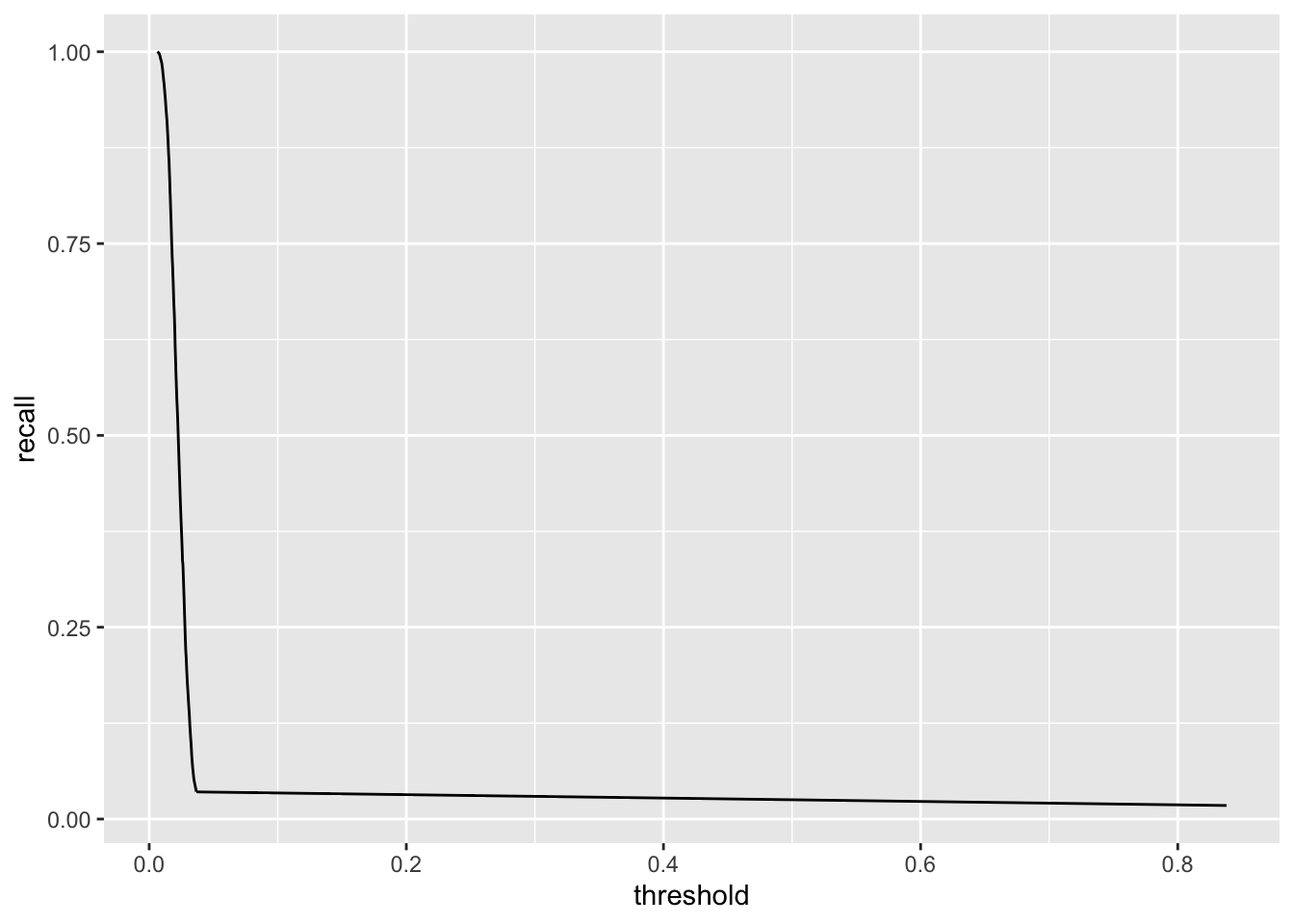
eval$roc() %>% 
collect() %>% 
    ggplot(aes(FPR, TPR)) +
    geom_line()

eval$recall_by_threshold() %>% 
    ggplot(aes(threshold, recall)) +
    geom_line()

eval$recall_by_threshold()

## # Source: spark<?> [?? x 2]
##    threshold recall
##        <dbl>  <dbl>
##  1    0.838  0.0177
##  2    0.0367 0.0356
##  3    0.0348 0.0514
##  4    0.0338 0.0667
##  5    0.0332 0.0799
##  6    0.0326 0.0960
##  7    0.0321 0.108 
##  8    0.0317 0.121 
##  9    0.0312 0.137 
## 10    0.0307 0.150 
## # … with more rows

8.52 Evaluating the model

Just try it on test data!

8.53 With this method there is a risk of overfitting

One alternative method is K-fold Cross Validation
Split the training data into K overlapping folds (subsets)
Train model on K different folds is more robust

8.54 There are different methods for cross validation

Depends on how much detail you want
The first and easiset is the in built method
The second is to write it yourself, which we will not cover in detail but I will provide some useful links

8.55 Inbuilt function

Requires a ml-pipeline

8.56 What the hell is an ml pipeline?

It is the true power of Spark
Once you fit a model with, e.g. ml_logistic_regression() a pipeline is created under the hood
They are a way to simplify you modelling and streamline the process
They are also unbearable for data engineers who can take your pipeline and put it into production
However, they differ from other modelling techniques in R

8.57 Pipeline vs pipeline model

Pipeline is just a sequence of tranformers and estimators
Pipeline model is a pipeline that has been trained

8.58 Create pipeline estimator

Easy with ml_pipeline()

pipeline <- ml_pipeline(sc) %>% 
  ft_standard_scaler(
    input_col = "features",
    output_col = "features_scaled", 
    with_mean = TRUE)

pipeline

## Pipeline (Estimator) with 1 stage
## <pipeline_2df7344fb657> 
##   Stages 
##   |--1 StandardScaler (Estimator)
##   |    <standard_scaler_2df75d4c2495> 
##   |     (Parameters -- Column Names)
##   |      input_col: features
##   |      output_col: features_scaled
##   |     (Parameters)
##   |      with_mean: TRUE
##   |      with_std: TRUE

8.59 Create pipeline transformer

df <- copy_to(sc, data.frame(value = rnorm(100000))) %>% 
  ft_vector_assembler(input_cols = "value", output_col = "features")

ml_fit(pipeline, df)

## PipelineModel (Transformer) with 1 stage
## <pipeline_2df7344fb657> 
##   Stages 
##   |--1 StandardScalerModel (Transformer)
##   |    <standard_scaler_2df75d4c2495> 
##   |     (Parameters -- Column Names)
##   |      input_col: features
##   |      output_col: features_scaled
##   |     (Transformer Info)
##   |      mean:  num -0.000527 
##   |      std:  num 1

8.60 Creating a model pipeline

With the old faithful r-formula

pipeline <- ml_pipeline(sc) %>%
  ft_r_formula(churn ~ total_charges_log + monthly_charges_log + senior_citizen + partner + 
        tenure + phone_service + multiple_lines + internet_service + online_security +
        online_backup + device_protection + tech_support + streaming_tv +
        streaming_movies + contract + paperless_billing + payment_method) %>%
  ml_logistic_regression()

pipeline

## Pipeline (Estimator) with 2 stages
## <pipeline_2df7768f1d71> 
##   Stages 
##   |--1 RFormula (Estimator)
##   |    <r_formula_2df72dd62286> 
##   |     (Parameters -- Column Names)
##   |      features_col: features
##   |      label_col: label
##   |     (Parameters)
##   |      force_index_label: FALSE
##   |      formula: churn ~ total_charges_log + monthly_charges_log + senior_citizen + partner + tenure + phone_service + multiple_lines + internet_service + online_security + online_backup + device_protection + tech_support + streaming_tv + streaming_movies + contract + paperless_billing + payment_method
##   |      handle_invalid: error
##   |      stringIndexerOrderType: frequencyDesc
##   |--2 LogisticRegression (Estimator)
##   |    <logistic_regression_2df74574a2ec> 
##   |     (Parameters -- Column Names)
##   |      features_col: features
##   |      label_col: label
##   |      prediction_col: prediction
##   |      probability_col: probability
##   |      raw_prediction_col: rawPrediction
##   |     (Parameters)
##   |      aggregation_depth: 2
##   |      elastic_net_param: 0
##   |      family: auto
##   |      fit_intercept: TRUE
##   |      max_iter: 100
##   |      reg_param: 0
##   |      standardization: TRUE
##   |      threshold: 0.5
##   |      tol: 1e-06

8.61 `ml_cross_validator`-function

Main purpose is hyperparameter tuning, i.e. model selection
Evaluates a grid with different values

grid <- list(logistic_regression = list(elastic_net_param = 0, reg_param = 0))

8.62 `ml_cross_validator`-function

cv <- ml_cross_validator(
  sc,
  estimator = pipeline, # use our pipeline to estimate the model
  estimator_param_maps = grid, # use the params in grid
  evaluator = ml_binary_classification_evaluator(sc, metric_name = "areaUnderPR"), # how to evaluate the CV
  num_folds = 10, # number of CV folds
  seed = 2018
)

cv

## CrossValidator (Estimator)
## <cross_validator_2df729de609f> 
##  (Parameters -- Tuning)
##   estimator: Pipeline
##              <pipeline_2df7768f1d71> 
##   evaluator: BinaryClassificationEvaluator
##              <binary_classification_evaluator_2df7257ce213> 
##     with metric areaUnderPR 
##   num_folds: 10 
##   [Tuned over 1 hyperparameter set]

cv_model <- ml_fit(cv, telco_train)

And evaluate

cv_model <- ml_load(sc, "models/cv_model_log_telco")

cv_model$avg_metrics_df

##   areaUnderPR elastic_net_param_1 reg_param_1
## 1   0.6763331                   0           0

8.62.1 Excercise

Make sure your feature engineered table is saved with sdf_register()
Instead of data use ml_pipeline(sc) as your first step, then specify your formula with ft_r_formula() and lastly apply ml_logistic_regression() and save it as a pipeline
Save a grid list(logistic_regression = list(elastic_net_param = 0, reg_param = 0))
Use the inbuilt Cross Validation function to train your model on 5 folds
What metric do you use to evaluate the model? Check ?ml_binary_classification_evaluator() to see what metrics are available.
How does this result differ from your previous result?

pipeline <- ml_pipeline(sc) %>%
    ft_r_formula(label ~ ft_scaled + age_quant) %>% 
    ml_logistic_regression()

grid <- list(logistic_regression = list(elastic_net_param = c(0), reg_param = c(0)))

cv_model <- ml_load(sc, "models/glr_model_cv")

cv <- ml_cross_validator(
  sc,
  estimator = pipeline, # use our pipeline to estimate the model
  estimator_param_maps = grid, # use the params in grid
  evaluator = ml_binary_classification_evaluator(sc, metric_name = "areaUnderPR"),  # how to evaluate the CV
  num_folds = 5, # number of CV folds
  seed = 2018
)

cv_model <- ml_fit(cv, data_train_scaled)

And evaluate it:

cv_model$avg_metrics_df

##   areaUnderPR elastic_net_param_1 reg_param_1
## 1  0.02764648                   0           0

8.63 Other models

Models that are included in the sparklyr package can be found: https://spark.rstudio.com/mlib/
For more details on how the models work: https://spark.apache.org/docs/latest/ml-classification-regression.html

8.64 Train and tune a random forest

pipeline_telco <- ml_pipeline(sc) %>%
  ft_r_formula(churn ~ log_charges + senior_citizen + partner + 
        tenure + phone_service + multiple_lines + internet_service + online_security +
        online_backup + device_protection + tech_support + streaming_tv +
        streaming_movies + contract + paperless_billing + payment_method) %>%
  ml_random_forest_classifier()

pipeline_telco

## Pipeline (Estimator) with 2 stages
## <pipeline_2df7504740cd> 
##   Stages 
##   |--1 RFormula (Estimator)
##   |    <r_formula_2df775ef7be7> 
##   |     (Parameters -- Column Names)
##   |      features_col: features
##   |      label_col: label
##   |     (Parameters)
##   |      force_index_label: FALSE
##   |      formula: churn ~ log_charges + senior_citizen + partner + tenure + phone_service + multiple_lines + internet_service + online_security + online_backup + device_protection + tech_support + streaming_tv + streaming_movies + contract + paperless_billing + payment_method
##   |      handle_invalid: error
##   |      stringIndexerOrderType: frequencyDesc
##   |--2 RandomForestClassifier (Estimator)
##   |    <random_forest_classifier_2df73dafb72e> 
##   |     (Parameters -- Column Names)
##   |      features_col: features
##   |      label_col: label
##   |      prediction_col: prediction
##   |      probability_col: probability
##   |      raw_prediction_col: rawPrediction
##   |     (Parameters)
##   |      cache_node_ids: FALSE
##   |      checkpoint_interval: 10
##   |      feature_subset_strategy: auto
##   |      impurity: gini
##   |      max_bins: 32
##   |      max_depth: 5
##   |      max_memory_in_mb: 256
##   |      min_info_gain: 0
##   |      min_instances_per_node: 1
##   |      num_trees: 20
##   |      seed: 207336481
##   |      subsampling_rate: 1

grid <- list(
  random_forest = list(
    num_trees = c(60, 100, 150, 200, 500),
    impurity = c("gini")
  )
)

pipeline_telco <- ml_pipeline(sc) %>%
  ft_r_formula(churn ~ log_charges + senior_citizen + partner + 
        tenure + phone_service + multiple_lines + internet_service + online_security +
        online_backup + device_protection + tech_support + streaming_tv +
        streaming_movies + contract + paperless_billing + payment_method) %>%
  ml_random_forest_classifier()

cv <- ml_cross_validator(
  sc,
  estimator = pipeline_telco, # use our pipeline to estimate the model
  estimator_param_maps = grid, # use the params in grid
  evaluator = ml_binary_classification_evaluator(sc, metric_name = "areaUnderPR"),  # how to evaluate the CV
  num_folds = 5, # number of CV folds
  seed = 2018
)

cv_model <- ml_fit(cv, telco_train)

cv_model <- ml_load(sc, "models/cv_model_rf_tune")

cv_model$avg_metrics_df

##   areaUnderPR impurity_1 num_trees_1
## 1   0.6485323       gini          60
## 2   0.6488818       gini         100
## 3   0.6479653       gini         150
## 4   0.6513677       gini         200
## 5   0.6475676       gini         500

8.65 Train a model with random forest on your data

Tune num_trees_1
Use a maximum of three grids for num trees, e.g. c(50, 100, 200), this might take a couple of minutes
Use 3 folds
Evaluate the model

pipeline <- ml_pipeline(sc) %>%
    ft_r_formula(label ~ ft_scaled + age_quant) %>% 
    ml_random_forest_classifier()

grid <- list(
  random_forest = list(
    num_trees = c(50, 100, 200),
    impurity = c("gini")
  )
)

cv <- ml_cross_validator(
  sc,
  estimator = pipeline, # use our pipeline to estimate the model
  estimator_param_maps = grid, # use the params in grid
  evaluator = ml_binary_classification_evaluator(sc, metric_name = "areaUnderPR"),  # how to evaluate the CV
  num_folds = 3, # number of CV folds
  seed = 2018
)

cv_model <- ml_fit(cv, data_train_scaled)

And evaluate

cv_model <- ml_load(sc, "models/cv_model_rf")

cv_model$avg_metrics_df

##   areaUnderPR impurity_1 num_trees_1
## 1  0.03515766       gini          50
## 2  0.03531436       gini         100
## 3  0.03579500       gini         200

8.66 Feature importance

rf <- ml_random_forest_classifier(
    telco_train,
    churn ~ total_charges_log + monthly_charges_log + senior_citizen + partner + #<<
        tenure + phone_service + multiple_lines + internet_service + online_security +
        online_backup + device_protection + tech_support + streaming_tv +
        streaming_movies + contract + paperless_billing + payment_method,
    num_trees = 200, impurity = "gini"
    )

p <- ml_tree_feature_importance(rf) %>% 
    ggplot(aes(x = reorder(feature, importance), y = importance)) +
    geom_col() +
    coord_flip()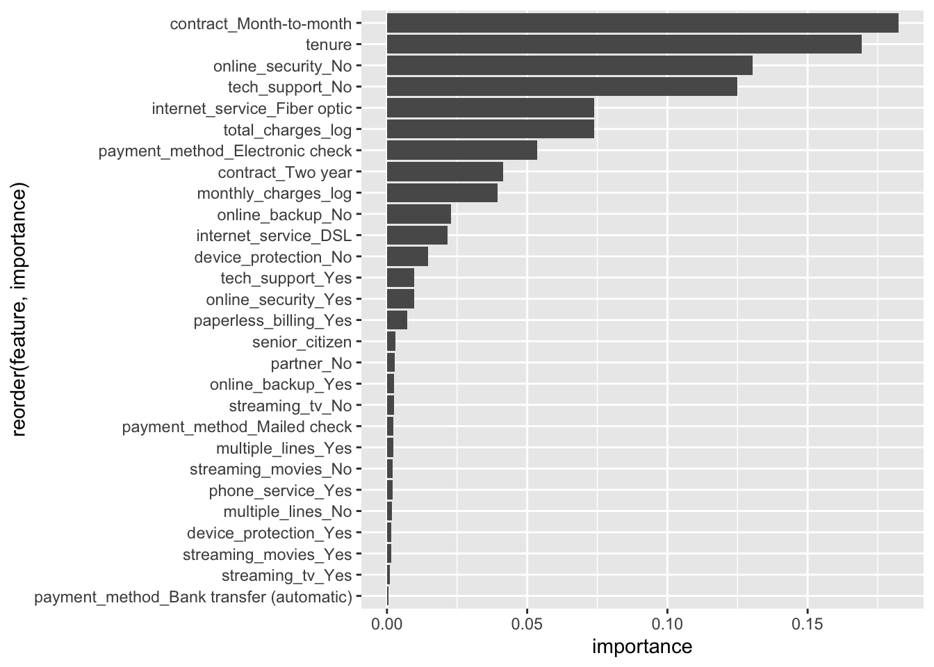

rf<- ml_random_forest_classifier(
    telco_train,
    churn ~ total_charges_log + monthly_charges_log + senior_citizen + partner + #<<
        tenure + internet_service + online_security +
        online_backup + device_protection + tech_support + streaming_tv +
        streaming_movies + contract + paperless_billing + payment_method,
    num_trees = 200, impurity = "gini"
    )

p <- ml_tree_feature_importance(rf) %>% 
    ggplot(aes(x = reorder(feature, importance), y = importance)) +
    geom_col() +
    coord_flip()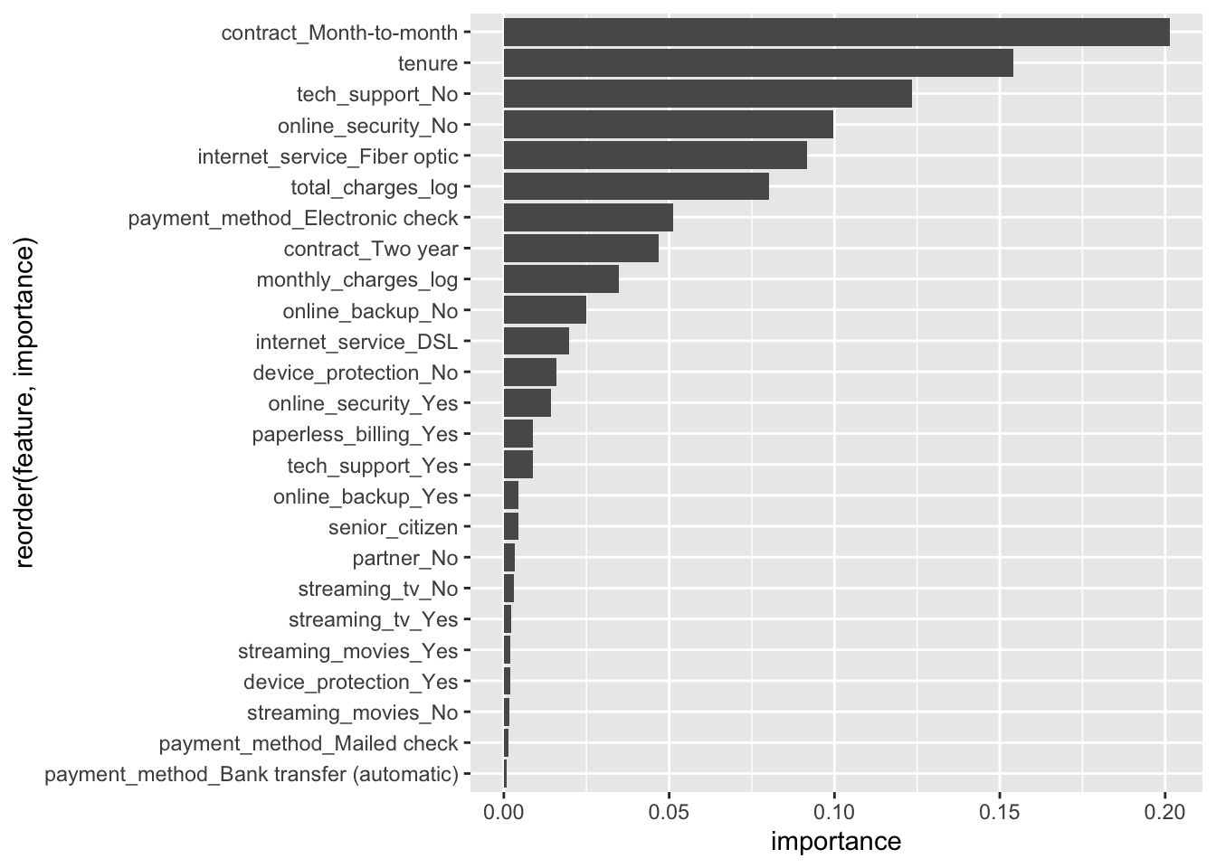

rf_simple <- ml_random_forest_classifier(
    telco_train,
    churn ~ total_charges_log + monthly_charges_log + senior_citizen + partner + #<<
        tenure + internet_service + online_security +
        online_backup + device_protection + tech_support + streaming_tv +
        streaming_movies + contract + paperless_billing + payment_method,
    num_trees = 200, impurity = "gini"
    )

rf<- ml_random_forest_classifier(
    telco_train,
    churn ~ total_charges_log + monthly_charges_log + senior_citizen + partner + #<<
        tenure + phone_service + multiple_lines + internet_service + online_security +
        online_backup + device_protection + tech_support + streaming_tv +
        streaming_movies + contract + paperless_billing + payment_method,
    num_trees = 200, impurity = "gini"
    )

ml_binary_classification_evaluator(ml_predict(rf_simple, telco_train), metric_name = "areaUnderROC")

## [1] 0.8517093

ml_binary_classification_evaluator(ml_predict(rf, telco_train), metric_name = "areaUnderROC")

## [1] 0.8520151

8.66.1 Excercise

Use your tuned parameter in from your cross validation of random forest
Create a random forest model using ml_random_forest_classifier(), that is not using a pipeline
Take a look at your feature importance of your random forest classifier

rf <- ml_random_forest_classifier(data_train_scaled, label ~ avg_monthly_data_usage + number_of_events +
                                                                                                                                                days_with_price_plan +  days_with_contract +
                                                                                                                                                days_since_price_plan_launch+ 
                                                                                                                                                hardware_age_imp + cpe_model_days_in_net_imp +
                                                                                                                                            age_quant_oh,
                                                                                                                                        num_trees = 100, impurity = "gini")

ml_tree_feature_importance(rf) %>% 
    ggplot(aes(x = reorder(feature, importance), y = importance)) +
    geom_col() +
    coord_flip()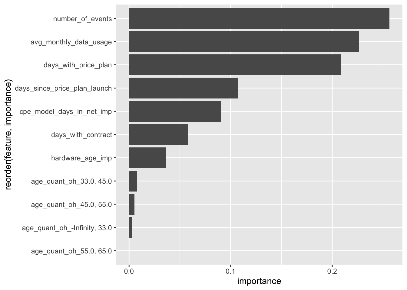

8.67 How to handle imbalance?

Three common techniques:
Oversampling
Undersampling
Create synthetic new observations

8.68 Undersampling

balance <- telco_train %>% 
    group_by(churn) %>% 
    count() %>% 
    ungroup() %>% 
    mutate(freq = n / sum(n)) %>% 
    collect()

## Warning: Missing values are always removed in SQL.
## Use `SUM(x, na.rm = TRUE)` to silence this warning
## This warning is displayed only once per session.

balance

## # A tibble: 2 x 3
##   churn     n  freq
##   <chr> <dbl> <dbl>
## 1 No     4118 0.734
## 2 Yes    1493 0.266

sratio <- balance[,2][[1]][[2]] / balance[,2][[1]][[1]]

telco_train_maj <- filter(telco_train, churn == "No")
telco_train_min <- filter(telco_train, churn == "Yes")

telco_train_maj_samp <- sdf_sample(telco_train_maj, fraction = sratio)

telco_train_unders <- sdf_bind_rows(telco_train_maj_samp, telco_train_min) %>% 
    sdf_register("telco_data_unders")

telco_train_unders %>% 
                            group_by(churn) %>% 
    count() %>% 
    ungroup() %>% 
    mutate(freq = n / sum(n)) %>% 
    collect()

## # A tibble: 2 x 3
##   churn     n  freq
##   <chr> <dbl> <dbl>
## 1 No     1505 0.502
## 2 Yes    1493 0.498

rf_under_telco <- ml_random_forest_classifier(telco_train_unders, 
                                                                                                                                                                                        churn ~ monthly_charges_log + senior_citizen + partner + 
        tenure + phone_service + multiple_lines + internet_service + online_security +
        online_backup + device_protection + tech_support + streaming_tv +
        streaming_movies + contract + paperless_billing + payment_method, 
        num_trees = 200, impurity = "gini")

rf_telco <- ml_random_forest_classifier(telco_train,
                                                                                                                                                                churn ~ monthly_charges_log + senior_citizen + partner + 
        tenure + phone_service + multiple_lines + internet_service + online_security +
        online_backup + device_protection + tech_support + streaming_tv +
        streaming_movies + contract + paperless_billing + payment_method, 
        num_trees = 200, impurity = "gini")

ml_binary_classification_evaluator(ml_predict(rf_under_telco, telco_train), metric_name = "areaUnderROC")

## [1] 0.8497889

ml_binary_classification_evaluator(ml_predict(rf_telco, telco_train), metric_name = "areaUnderROC")

## [1] 0.8498909

8.69 Apply undersampling to your data set and evaluate a random forest model

Use ml_random_forest_classifier() and not a pipeline

balance <- data_train %>% 
                            group_by(label) %>% 
    count() %>% 
    ungroup() %>% 
    mutate(freq = n / sum(n)) %>% 
    collect()

balance

## # A tibble: 2 x 3
##   label      n   freq
##   <int>  <dbl>  <dbl>
## 1     0 185947 0.980 
## 2     1   3791 0.0200

sratio <- balance[,2][[1]][[2]] / balance[,2][[1]][[1]]

data_train_maj <- filter(data_train_scaled, label == 0)
data_train_min <- filter(data_train_scaled, label == 1)

data_train_maj_samp <- sdf_sample(data_train_maj, fraction = sratio)

data_train_unders <- sdf_bind_rows(data_train_maj_samp, data_train_min) %>%
    sdf_register("data_train_unders")

data_train_unders %>% 
                            group_by(label) %>% 
    count() %>% 
    ungroup() %>% 
    mutate(freq = n / sum(n)) %>% 
    collect()

## # A tibble: 2 x 3
##   label     n  freq
##   <int> <dbl> <dbl>
## 1     0  3872 0.505
## 2     1  3791 0.495

rf_unders <- ml_load(sc, "models/rf_unders")

rf_unders <- ml_random_forest_classifier(data_train_unders, label ~ avg_monthly_data_usage + number_of_events +
                                                                                                                                                days_with_price_plan +  days_with_contract+
                                                                                                                                                days_since_price_plan_launch + 
                                                                                                                                                hardware_age_imp + cpe_model_days_in_net_imp +
                                                                                                                                            age_quant_oh,
                                                                                                                                        num_trees = 100, impurity = "gini")

And evaluate

ml_binary_classification_evaluator(ml_predict(rf_unders, data_train_scaled), metric_name = "areaUnderPR")

## [1] 0.03689627

8.70 Feature selection using cross validation

Feature selection using cross validation: https://www.eddjberry.com/post/2018-12-12-sparklyr-feature-selection/

8.71 Feature selection using cross validation

ft_ind <- function(tbl, input_col_name){
    ft_string_indexer(tbl, input_col = input_col_name, output_col = paste0(input_col_name, "_i")) %>% 
        ft_one_hot_encoder(input_col = paste0(input_col_name, "_i"), output_col = paste0(input_col_name, "_oh"))
}

telco_train_oh <- telco_train %>% 
    ft_ind("gender") %>% 
    ft_ind("partner") %>% 
    ft_ind("dependents") %>% 
    ft_ind("phone_service") %>% 
    ft_ind("multiple_lines") %>% 
    ft_ind("internet_service") %>% 
    ft_ind("online_security") %>% 
    ft_ind("online_backup") %>% 
    ft_ind("device_protection") %>% 
    ft_ind("tech_support") %>% 
    ft_ind("streaming_tv") %>% 
    ft_ind("streaming_movies") %>% 
    ft_ind("contract") %>% 
    ft_ind("paperless_billing") %>% 
    ft_ind("payment_method") %>% 
    mutate(churn = if_else(churn == "Yes", 1L, 0L)) %>% 
    select(churn, senior_citizen, total_charges_log, monthly_charges_log, tenure, contains("oh"))

get_feature_cols <- function(tbl, response, exclude = NULL) {
  
  # column names of the data
  columns <- colnames(tbl)
  
  # exclude the response/outcome variable and 
  # exclude from the column names
  columns[!(columns %in% c(response, exclude))]
}

ml_fit_cv <-
  function(sc, # Spark connection
           tbl, # tbl_spark
           model_fun, # modelling function
           label_col, # label/response/outcome columns
           feature_cols_exclude = NULL, # vector of features to exclude
           param_grid, # parameter grid
           seed = sample(.Machine$integer.max, 1) # optional seed (following sdf_partition)
           ) {
    
    # columns for the feature
    feature_cols <-
      get_feature_cols(tbl, label_col, feature_cols_exclude)
    
    # vector assembler
    tbl_va <- ft_vector_assembler(tbl,
                                   input_cols = feature_cols,
                                   output_col = "features")
    
    # estimator
    estimator <- model_fun(sc, label_col = label_col)
    
    # an evaluator
    evaluator <-
      ml_binary_classification_evaluator(sc, label_col = label_col)
    
    # do the cv
    ml_cross_validator(
      tbl_va,
      estimator = estimator,
      estimator_param_maps = param_grid,
      evaluator = evaluator,
      seed = seed
    )
  }

df_feature_selection <-
  data_frame(excluded_feature = get_feature_cols(telco_train_oh, 'churn'))

df_feature_selection

param_grid <- list(logistic_regression = list(elastic_net_param = 0))

df_feature_selection <- df_feature_selection %>%
  mutate(
    cv_fit = map(
      excluded_feature,
      ~ ml_fit_cv(
        sc,
        tbl = telco_train_oh,
        model_fun = ml_logistic_regression,
        label_col = 'churn',
        feature_cols_exclude = .x,
        param_grid = param_grid,
        seed = 2018
      )
    ),
    avg_metric = map_dbl(cv_fit, ~ .x$avg_metrics)
  )

cv_fit_full <- ml_fit_cv(
  sc, 
  telco_train_oh, 
  ml_logistic_regression, 
  'churn',
  param_grid = param_grid, 
  seed = 2018
)

df_feature_selection <- df_feature_selection %>%
  mutate(full_avg_metric = cv_fit_full$avg_metrics)

df_feature_selection <- read_rds("/Users/filipwastberg/Documents/ferrologic/r-utbildning-tele2/data/df_features.RDS")

p <- ggplot(df_feature_selection,
       aes(excluded_feature, avg_metric, fill = avg_metric)) +
  coord_cartesian(ylim = c(0.5, 1)) +
  geom_hline(aes(yintercept = full_avg_metric), linetype = 'dashed') +
  annotate(
    'text',
    x = 'total_charges_log',
    y = 0.8505,
    label = 'Full model',
    family = 'mono',
    alpha = .75,
    size = 3.5
  ) +
  geom_point(shape = 21, size = 2.5, show.legend = FALSE) +
  scale_fill_viridis_c(option = 'B', end = 0.9) +
  labs(
    x = 'Excluded feature',
    y = 'Average Area \nunder the ROC curve',
    title = 'Feature selection cross-validation',
    subtitle = 'Performance from removing each feature'
  ) +
  theme_minimal(base_size = 12, base_family = 'mono') +
  theme(panel.grid.major.x = element_blank()) +
    coord_flip()

## Coordinate system already present. Adding new coordinate system, which will replace the existing one.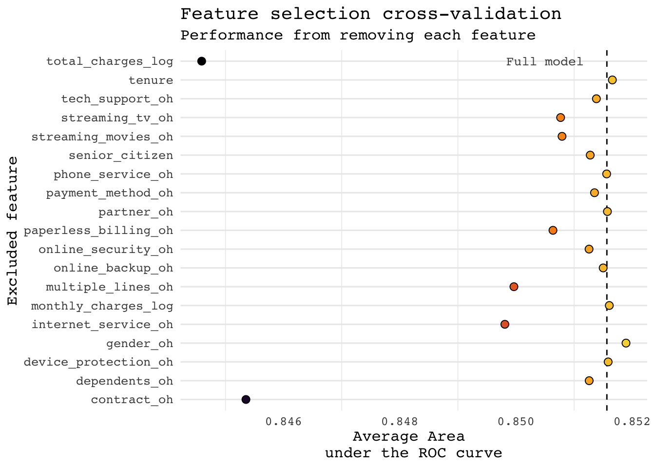

8.72 What about production?

Okey, so you have built a random forest model that you want to implement
You send it to an implementation engineer and ask when you can have it in production
In about 3 months because I have to write 500 if-else statements
With spark there are two main ways to put them in production:
Batch processing, i.e. scoring a number of rows at the same time
Real time predictions using an API

8.73 Batch processing

You just need some computer/server to host the scheduling of a R-script
Or an environment that administrates the clusters, e.g. Databricks, Zeppelin

8.74 Real time predictions using an API

APIs (application programming interfaces)

knitr::include_graphics("images/api.png")

8.75 API:s

knitr::include_graphics("images/api-request.png")

You can do this via R through the package plumber
https://www.rplumber.io/

knitr::include_graphics("images/plumber-broken.png")

8.76 Usually you use an implementation engineer

Either way you will have to save your model

8.77 Saving your model

Save the whole pipeline

ml_save(rf_telco, "models/rf_telco")

8.78 Using the mleap package

library(mleap)

input_columns <- get_feature_cols(telco_train_oh, "label")

telco_train_oh %>% 
    sdf_register("telco_data")

pipeline_telco <- ml_pipeline(sc) %>%
    ft_vector_assembler(input_cols = input_columns, "features") %>% 
  ml_random_forest_classifier(label_col = "churn", num_trees = 200)

telco_fit <- ml_fit(pipeline_telco, telco_train_oh)

ml_write_bundle(telco_fit, ml_transform(telco_fit, telco_train_oh),  path = "models/rf_telco.zip")

8.78.1 Excercise

Train your “final” model as a pipeline
Save your final model with ml_save()

8.79 Searching for help on spark and sparklyr

https://spark.rstudio.com/
https://spark.apache.org/docs/2.2.0/ml-guide.html
stackoverflow.com, #sparklyr, #pyspark #spark

Chapter 8 Exploratory data analysis and feature engineering

8.1 Big data

8.2 But what is it, really?

8.3 What is it not?

8.4 How can we use it in R?

8.5 Now… do you need it?

8.6 The Sparklyr API is really great

8.7 Set up your Spark context

8.8 We can manipulate our configuration

8.9 Okey, let’s load some data.

8.10 What’s the plan?

8.11 sdf_ functions

8.12 Exploratory analysis - one of the most important parts

8.13 Distribution of NA’s

8.14 If we want to do it for all variables

8.14.1 Excercise

8.15 EDA

8.16 Split the data

8.17 Continue in your Rmarkdown-file

8.18 Check out the correlations

8.18.1 Excercise

8.19 Ideally we want to calculate the probability that a customer will buy new hardware within 30 days

8.20 Feature engineering

8.21 What is feature engineering?

8.22 Some terminology that surely isn’t new to you

8.23 Sparklyr basics reminder

8.24 There are generally two ways that we can do feature engineering with sparklyr.

8.24.1 ExcerciseBut first let’s clean our data set a bit

8.25 Feature transformers

8.26 Imputations

8.27 How do we impute missing values for categorical variables?

8.28 Excerices

8.29 How to handle categories

8.30 Makes sense with data that is evenly distributed

8.31 You can use ft_string_indexer and ft_one_hot_encoder_estimator to create them manually

8.32 But what about when they are not evenly distributed?

8.32.1 Excercise

8.33 But what if you have a large number of categories?

8.34 Feature hashing

8.35 A word of caution

8.36 Numerical transformations

8.36.1 Excercise

8.37 Rescaling

8.38 Rescaling can improve some models

8.39 Before applying a scale function you need to assemble your vector

8.40 You can also scale with dplyr

8.40.1 Excercise

8.41 Bucketizing

8.41.1 Excercise

8.42 Dimensionality reduction

8.43 PCA

8.44 Interactions

8.44.1 sdf_register()

8.45 Last excercise

8.46 Modelling with sparklyr

8.47 ml_ functions

8.48 The feature engineering is done

8.49 Fitting models

8.50 Fitting a logistic regression

8.51 Evaluating the model

8.51.1 Excercise

8.52 Evaluating the model

8.53 With this method there is a risk of overfitting

8.54 There are different methods for cross validation

8.55 Inbuilt function

8.56 What the hell is an ml pipeline?

8.57 Pipeline vs pipeline model

8.58 Create pipeline estimator

8.59 Create pipeline transformer

8.60 Creating a model pipeline

8.61 ml_cross_validator-function

8.62 ml_cross_validator-function

8.62.1 Excercise

8.63 Other models

8.64 Train and tune a random forest

8.65 Train a model with random forest on your data

8.66 Feature importance

8.66.1 Excercise

8.67 How to handle imbalance?

8.68 Undersampling

8.11 `sdf_` functions

8.31 You can use `ft_string_indexer` and `ft_one_hot_encoder_estimator` to create them manually

8.47 `ml_` functions

8.61 `ml_cross_validator`-function

8.62 `ml_cross_validator`-function