Chapter 4 Calibration procedure
To perform the geographic assignment of samples of unknown origins (i.e. assignment samples), you need to produce an isoscape that describes how the isotope composition of source samples varies in space (see chapter 3). If the assignment samples are of different nature than the source samples (e.g. the source samples are precipitation water and the assignment samples are some animals), you will also need to account for such a discrepancy. Doing so is needed because looking at the isotopic composition in any candidate assignment location no longer reflects the isotopic composition of samples that may come from such a location (e.g. due to isotopic fractionation along the trophic chain).
In IsoriX, the function performing the calibration is called calibfit().
The goal of this function is to characterize the relationship between the isotopic composition of samples similar to those that you want to assign but of known origin (e.g. sedentary individuals) – which we call calibration samples – and the isotopic composition of the environment where these samples are collected.
During the assignment step (detailed in chapter 5), the relationship established by calibfit() will be used to rescale the mean isoscape so that it represents the isotopic composition of the samples to be assigned.
We call the statistical model behind the calibration the calibration model and the fitted model the calibration fit. In other publications, the latter is also referred to as the calibration function, calibration curve, or transfer function.
In IsoriX, the calibration fit predicts the isotopic composition of calibration samples from the isotopic composition of their environment.
Others sometimes do the reverse; that is, to perform their assignments they rely on a calibration fit predicting the isotopic composition of the environment from the isotopic composition of calibration samples.
Whatever term you may use to refer to the calibration in your paper (calibration fit, calibration function, calibration curve or transfer function), do make it clear for others in which direction the fit looks at the problem.
This matters because the direction dictates how the estimates associated with the fit can then be used to perform an assignment.
4.1 Choosing the calibration method
The data behind any calibration fit ultimately derive from the isotopic composition of calibration samples and that of the environment in the same (known) location.
Yet, because there are different ways to get these data, we introduced since IsoriX version 0.8.3 the possibility to choose among four alternatives to generate a calibration fit.
We call these methods ‘wild’, ‘lab’, ‘desk’ and ‘desk_inverse’.
It is important for you to understand which method is most appropriate for your utilization since different methods imply different assumptions which translate into different statistics used to perform the assignment step.
Different methods also require you to feed different type of data to calibfit().
The method ‘wild’ corresponds to the situation where the isotopic composition of calibration samples has been measured, while the isotopic composition of the environment where such samples were collected has not been so. This method thus infers the source isotope data corresponding to each calibration sample from the mean isoscape build in chapter 3.
We chose the method wild as the default method in calibfit() because most empiricists do not actually collect environmental samples at the locations of the calibration samples.
For this reason, we will also focus on this method in the rest of the workflow illustrated here.
Yet, let us give you a very brief summary of when to use the other methods since you may have a different research design.
The method ‘lab’ is the one to use in two main situations:
- you measured the isotopic composition of your calibration samples and you also know with great confidence the isotopic composition in their environment (either because you measured it or because your calibration individuals grew in a lab where the food and water has known isotopic composition).
- you measured nothing but want to use datapoints of a published calibration relationship.
While the method ‘wild’ and the method ‘lab’ both neglect measurement uncertainties, the ‘wild’ method does account for the fact that the isotopic composition at the location where the calibration samples have been collected is predicted with some (estimated) uncertainty. In contrast, the ‘lab’ method does not account for any uncertainty in the isotopic composition of the environment. An important corollary is that using the ‘lab’ method to recycle the calibration made by others comes at the cost of neglecting uncertainty in the isotopic composition of the environment.
The methods ‘desk’ and ‘desk_inverse’ are to be used in case you have no measurements of any isotopic composition, cannot deduce measurements from a published plot, and thus must rely on summary statistics (e.g. regression coefficients) found in a publication. The former (desk) can accept summary statistics from a model predicting the isotopic composition of the sample values from that of the environment. The latter (desk inverse) can accept summary statistics from a model predicting the isotopic composition of the environment from those of the calibration samples. Reliable assignments can be obtained using such methods provided that you supply all the summary statistics they require. If not, uncertainty terms will be neglected during the assignment step.
We can summarize when to use which method by a simple table:
| Method | Isotopic composition of the calibration samples | Isotopic composition of the environment associated with the calibration samples |
|---|---|---|
| wild | known | unknown, estimated from the isoscapes |
| lab | known | known, or assumed to be known |
| desk |
unknown, estimated from fit lm(sample_value ~ source_value)
|
unknown, estimated from fit lm(sample_value ~ source_value)
|
| desk_inverse |
unknown, estimated from fit lm(source_value ~ sample_value)
|
unknown, estimated from fit lm(source_value ~ sample_value)
|
When using a method other than the default method, you must set the method to be used by calibfit() using a specific argument called method, e.g. calibfit(..., method = 'lab').
More detailed information on the alternative calibration methods, the data they require and examples are available in the documentation of the function fitting the calibration model (see ?calibfit()).
4.2 Preparing the data (method ‘wild’)
Obtaining good data for the calibration fit is very important for obtaining a precise assignment. You should aim for data as close as possible to the following ideal situation:
The data are from many calibration samples covering the entire assignment area. Thus your data should span the whole range of each covariate considered in the models, which should limit risks associated with extrapolation when using the fitted calibration model during the geographic assignment.
The data correspond to many repeated measurements per location, which allows for a reliable estimation of the inter-sample variance in isotopic composition. Such variance captures the effect of biological variation in the isotopic signature of the calibration samples at each site.
The timing of the sampling events for the calibration samples matches the overall sampling period of the source isotope data.
The data are collected from samples directly comparable to those that need to be assigned; such as organisms from the same species and the same physiological state.
As an example, we will use here the calibration dataset CalibDataBatRev that is provided with IsoriX. This dataset contains stable isotope ratios of the non-exchangeable portion of hydrogen in fur keratin of non-migratory bats sampled across Europe:
| site_ID | long | lat | elev | sample_ID | species | sample_value |
|---|---|---|---|---|---|---|
| site_29 | 18.87101 | 46.19747 | 90 | 1 | 4 | -31.00384 |
| site_29 | 18.87101 | 46.19747 | 90 | 2 | 4 | -57.50992 |
| site_29 | 18.87101 | 46.19747 | 90 | 3 | 4 | -28.57132 |
| site_29 | 18.87101 | 46.19747 | 90 | 4 | 4 | -57.42604 |
| site_32 | 19.10489 | 48.53405 | 522 | 5 | 4 | -48.19924 |
| site_32 | 19.10489 | 48.53405 | 522 | 6 | 4 | -56.33560 |
For your own applications, make sure that the dataset you use has the same structure. That is, the calibration dataset must contain (as long as you use the calibration method ‘wild’) a column site_ID of class ‘factor’ describing the sampling site, the columns containing all covariates required for the geostatistical models to predict the isoscape values at these locations (so here long, lat, and elev), and a column sample_value containing the measured isotope values of the calibration samples. An important constraint to keep in mind is that only measurements on multiple calibration samples per location can capture variation between different samples exposed to the same isotope environment. Therefore, IsoriX needs multiple calibration samples for several (not necessarily all) sampling locations. That means that some levels of site_ID must be repeated on several rows. If laboratory measurements are replicated, we recommend to consider the mean measurement value for each sampling unit (here for each bat) instead of considering multiple rows for a given calibration sample in order to avoid confounding biological replicates from technical ones. If you do so, note however that this implies the technical variance to be neglected (which should be fine because it is usually very low unless something went wrong in the lab).
4.3 Fitting the calibration model (method ‘wild’)
With the calibration data at hand, we can thus proceed to fit the calibration model using calibfit():
To display the result of the calibration fit, you can simply type the name of the object we just created:
##
## Fixed effect estimates of the calibration fit
## sample_value = intercept + slope * mean_source_value + corrMatrix(1|site_ID) + slope^2 * (1|site_ID) + Error
##
##            intercept (+/- SE) = 3.20 +/- 4.40
##            slope     (+/- SE) = 0.77 +/- 0.08
##
## [for more information, use summary()]
The model formula will differ depending on the calibration method you used.
Here, for the method ‘wild’, the calibration model that is fitted is a particular Linear Mixed-effects Model (LMM). The particularity lies in the calibration model controlling for the uncertainty of the isoscape predictions.
The function calibfit() not only considers the prediction variance associated with each prediction from the mean model (which varies spatially) but also the prediction covariances between the different predictions of the isotope values across the isoscape.
Moreover, the variation between calibration samples is captured by the residual variance of the calibration fit.
You can also plot the calibration fit:
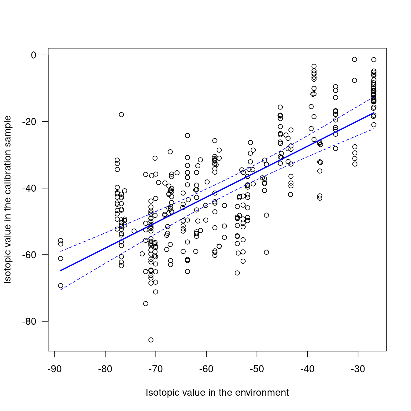
The plot illustrates a strong assumption made while fitting the calibration model: we consider that the relationship between the isotope values of the calibration samples and those of the environment are linearly related. For the moment, we offer no alternative to this assumption.