Chapter 6 Advanced usage
Chapters 3, 4 & 5 illustrated a simple workflow, but IsoriX allows for much more complex workflows.
The goal of this chapter is to illustrate such possibilities.
6.1 Working with plots
6.1.1 Lattice? No thanks, I want to use ggplot!
If lattice is not for you and you are more familiar with ggplot2, you can use it.
We did not implement specific functions for doing so, but since IsoriX spatial objects are now made with terra, it is relatively straightforward.
Here, is a first example using the recent package tidyterra which creates a plot of the mean isoscape:
##
## Attaching package: 'tidyterra'
## The following object is masked from 'package:kableExtra':
##
## group_rows## The following object is masked from 'package:stats':
##
## filter##
## Attaching package: 'ggplot2'## The following object is masked from 'package:IsoriX':
##
## layerggplot() +
geom_spatraster(data = EuropeIsoscape$isoscapes$mean) +
geom_spatvector(data = CountryBorders, fill = NA, colour = "white") +
geom_spatvector(data = OceanMask, fill = "lightgrey", colour = NA) +
scale_fill_binned(type = "viridis") +
scale_x_continuous(expand = c(0, 0), limits = c(-30, 60)) +
scale_y_continuous(expand = c(0, 0), limits = c(30, 70)) +
labs(fill = getOption_IsoriX("title_delta_notation"))## <SpatRaster> resampled to 500160 cells.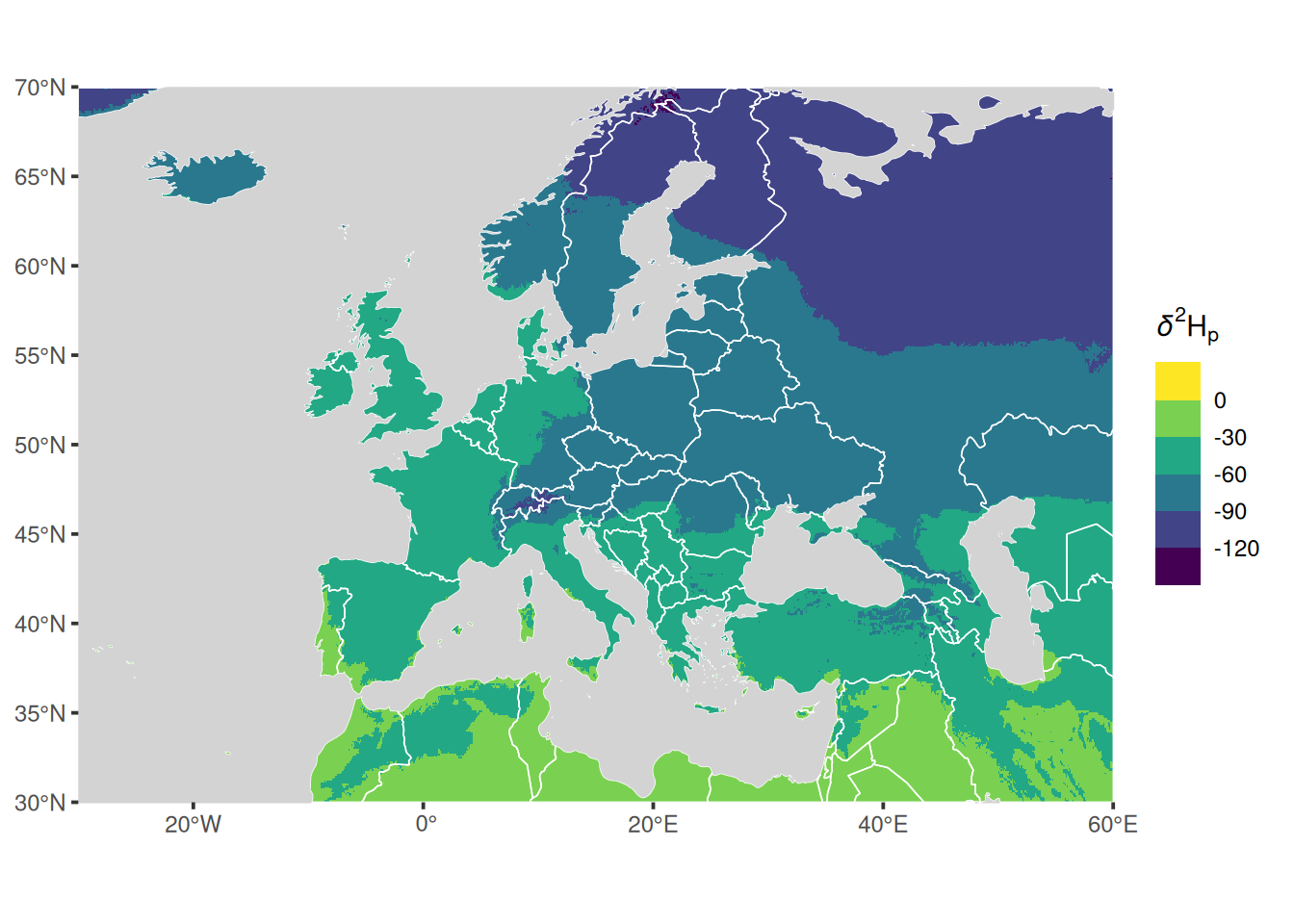
Here is the same thing not using tidyterra but instead converting the IsoriX objects on the fly into sf objects (for SpatVector) and into stars objects (for SpatRaster):
library(stars)
library(sf)
library(ggplot2)

ggplot() +
  geom_stars(data = st_as_stars(EuropeIsoscape$isoscapes$mean)) +
  geom_sf(data = st_as_sf(CountryBorders), fill = NA, colour = "white") +
  geom_sf(data = st_as_sf(OceanMask), fill = "lightgrey", colour = NA) +
  scale_fill_binned(type = "viridis") +
  scale_x_continuous(expand = c(0, 0), limits = c(-30, 60)) +
  scale_y_continuous(expand = c(0, 0), limits = c(30, 70)) +
  labs(fill = getOption_IsoriX("title_delta_notation"))
## Warning: Removed 81767 rows containing missing values or values outside the
## scale range (`geom_raster()`).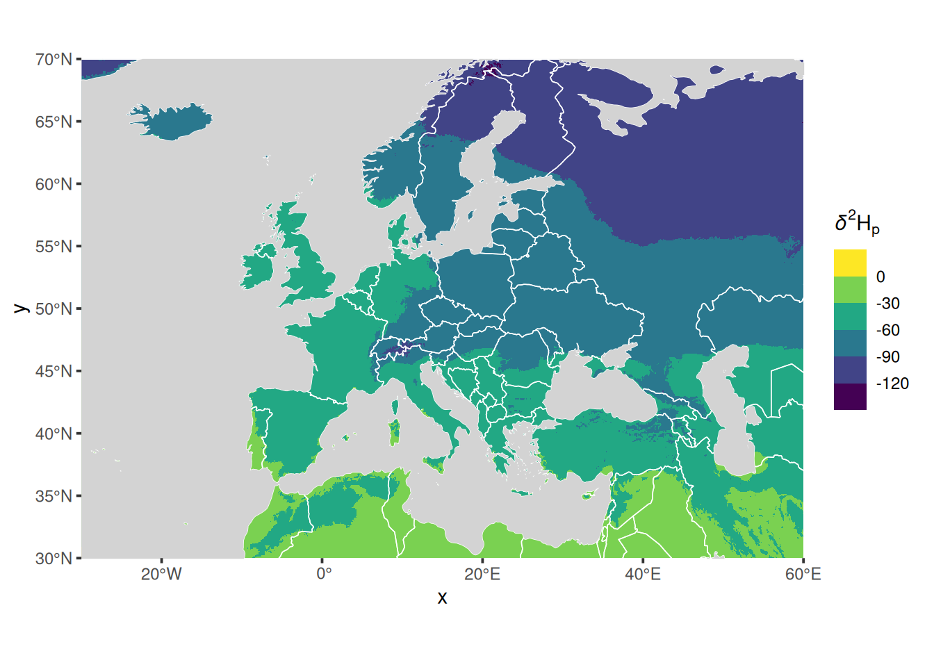
The benefit of using the combination ggplot2, sf & stars (as opposed to using tidyterra or even, alas, the functions of IsoriX) is that you will find plenty more tutorials online for how to draw nice maps that way.
Since tidyterra and ggplot2 have both overridden functions that IsoriX or this bookdown rely on, let’s unload these packages to avoid issues:
6.1.2 Fiddling with IsoriX plotting functions
If you do want to use our IsoriX plotting functions, note that it is possible to change pretty much anything on the existing plot; have a look at ?plots.
The help file should provide you with all the details you need to customize your plots.
Here are a couple of examples:
plot(EuropeIsoscape,
sources = list(pch = 3, col = "orange"),
borders = list(col = "white"),
mask = list(fill = "lightgrey"),
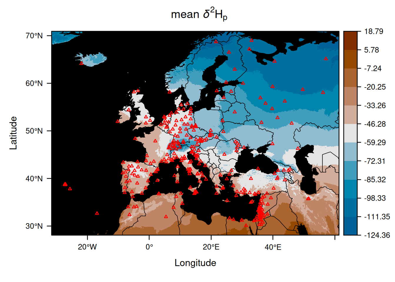
palette = list(range = c(-130, 10), step = 1, n_labels = 10, fn = "rainbow"))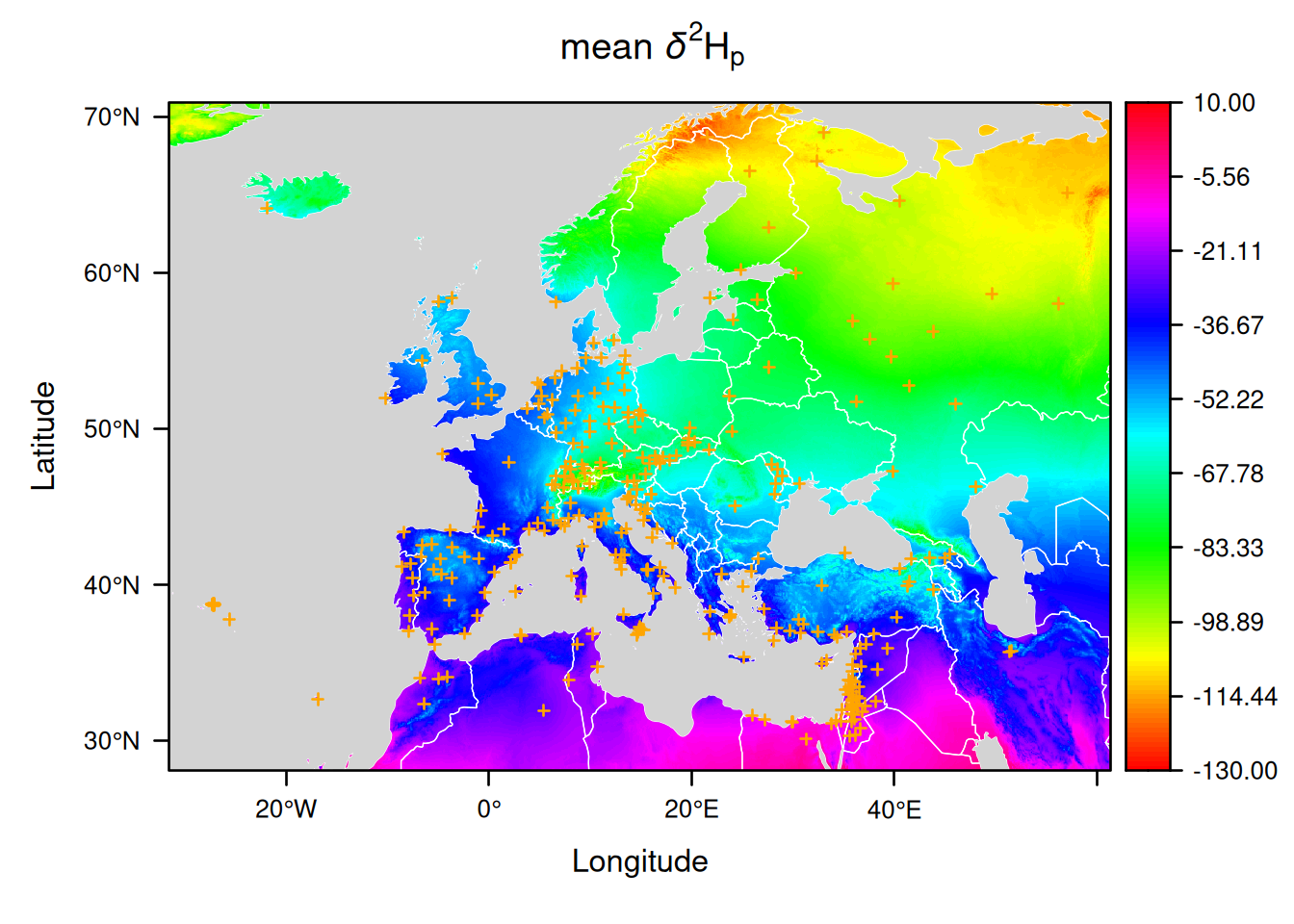
You can see that it is possible to provide a function defining the colors using the argument fn from the list palette.
Note that when it is set to NULL, the famous palette viridis is used instead of our default palette.
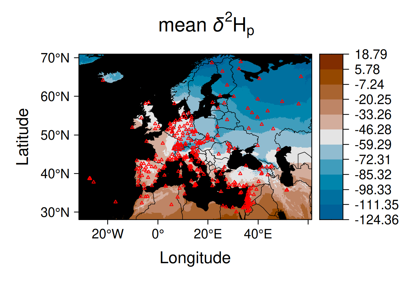
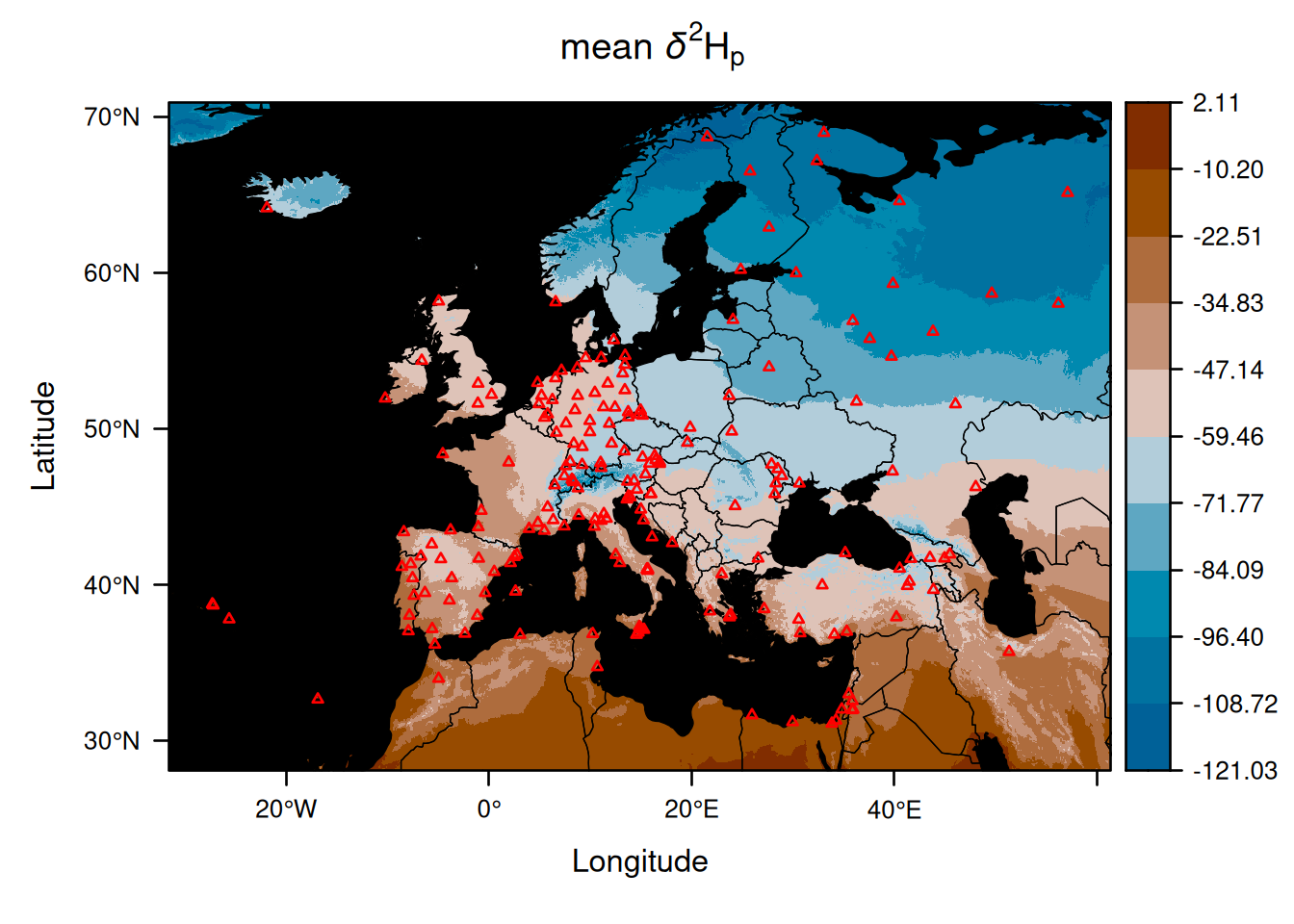
So here is another example, using such a palette:
plot(EuropeIsoscape,
     y_title = list(title = "H Isoscape"),
     sources = list(draw = FALSE),
     borders = list(borders = NULL),
     mask    = list(fill = "black"),
palette = list(range = c(-130, 20), step = 30, fn = NULL)) 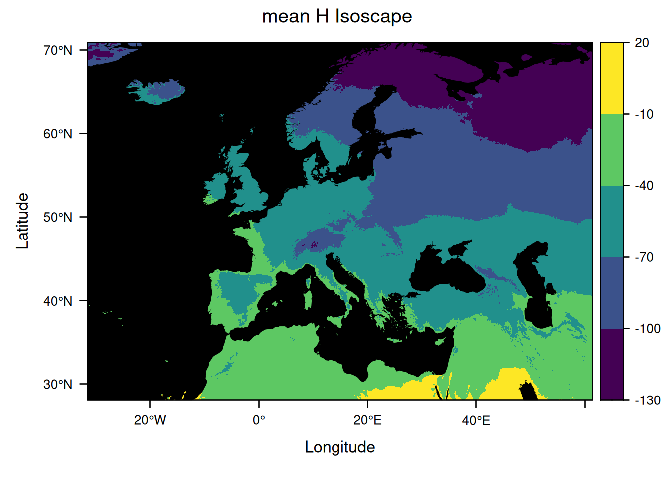
If you need to change things on the plots that are not covered by the plotting functions from IsoriX, it may be worth getting the basics of how to use lattice.
The package lattice is very powerful but not always very intuitive to use, so we are going to list here a few tips.
The easiest way to modify a plot is to start saving the plot into an object:
Then, the (generic) function update() allows you to change many aspects of the plot whenever applied to your plot object (here isoscape_plot).
For example, you can increase the size of the text in the previous plot as follows:
As an entry point to see what can be changed in a lattice plot, you should consult the help page that shows up when typing ?lattice::xyplot in your R console.
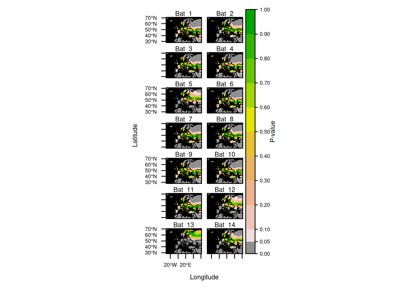
Multipanel plots created after assignments can be modified using the same principle. For example, you can rename the title of each panel and modify the organisation of the panels as follows:
assignment_plot <- plot(AssignedBats,
                        who = 1:14,
                        sources = list(draw = FALSE),
                        calibs = list(draw = FALSE),
                        assigns = list(draw = FALSE)
                        )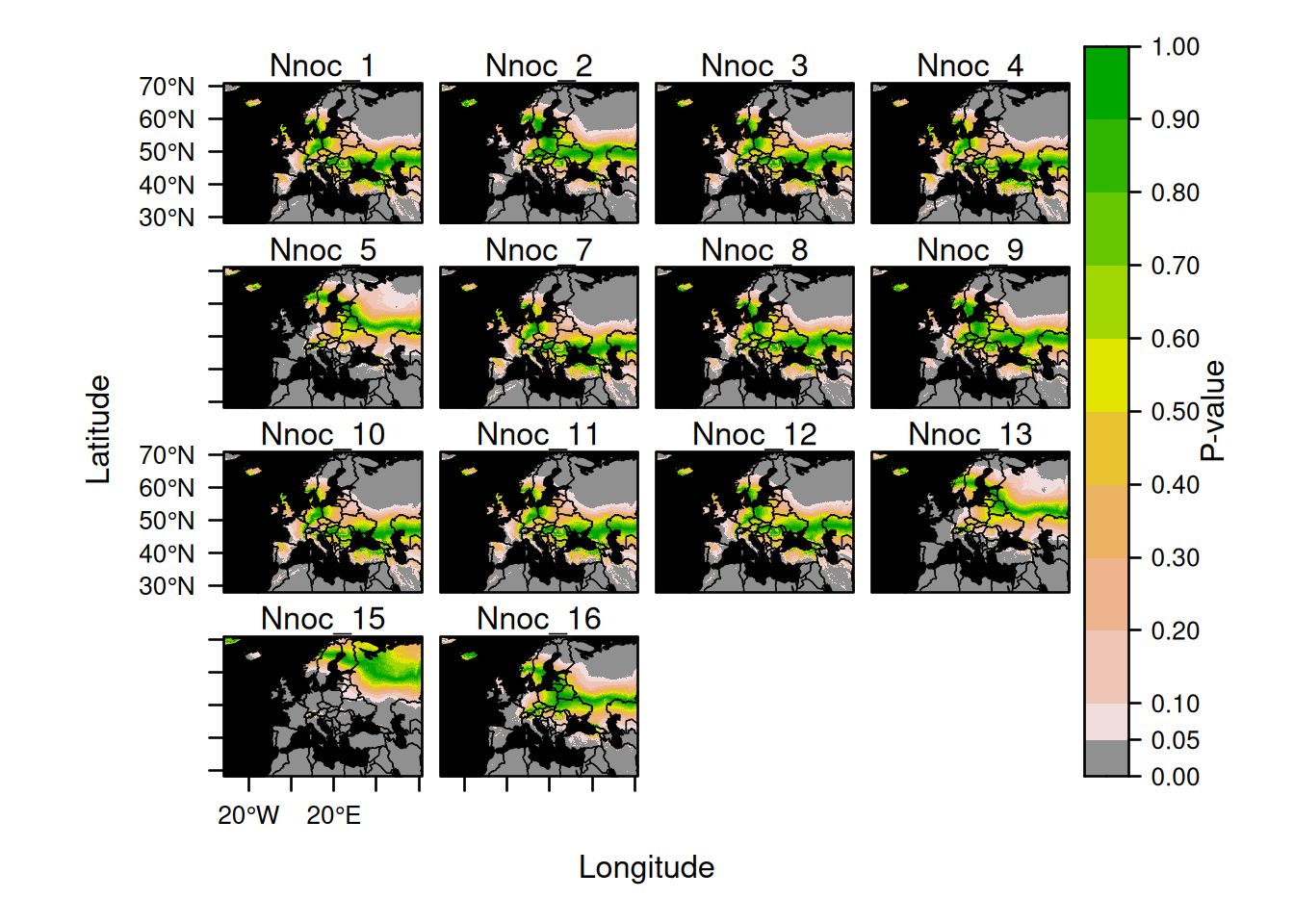
update(assignment_plot,
       par.settings = list(fontsize = list(text = 8)),
       strip = lattice::strip.custom(factor.levels = paste("Bat ", 1:14)),
       layout = c(col = 2, row = 7)
       )
If you want to add things on top of the plots, you can do it as you would do it for any plot created using lattice.
For example, consider you want to add the point that is the most compatible with the unknown origin of bats (see chapter 5).
The first step is to recover the coordinates for such a point:
library(terra)
coord <- crds(AssignedBats2$group$pv)
MaxLocation <- coord[which.max(values(AssignedBats2$group$pv)), ]
Maximum <- data.frame(long = MaxLocation[1], lat = MaxLocation[2])
Maximum
We can then plot this information on top of the assignment plot by simply typing:
plot(AssignedBats2, who = "group", plot = FALSE) +
  xyplot(Maximum$lat ~ Maximum$long, pch = 13, col = "orange", cex = 5, lwd = 2)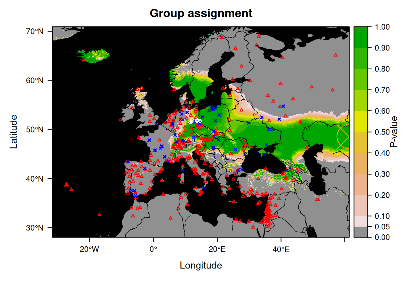
Note that the new symbol is present on the right edge of the plot.
6.1.3 Why you should save plots & how to export nice looking plots
Displaying the plot directly using R is very inefficient when it comes to high resolution isoscapes. It may take a very long time and it may not fully work.
It is better to directly plot the figures into files.
Geeky note: Since the lattice system is not part of ggplot2, the function ggsave() should not be used (unless you are really using ggplot2 as shown in section 6.1.1).
6.1.3.1 Using base R graphics devices functions
A first option is to save your plot using one of the base R functions such as png() or tiff().
For example, you could do:
png(filename = "output/Myisoscape.png",
    width = 1920,
    height = 1080,
    res = 200)
plot(EuropeIsoscape)
dev.off()
or
tiff(filename = "output/Myisoscape.tiff",
     width = 1920,
     height = 1080,
     res = 200)
plot(EuropeIsoscape)
dev.off()
As you can see, you first initialize the creation of the plot with the function png() or tiff(), then you call your plot, then you tell your computer that you are done with dev.off().
As arguments, you probably want to specify the dimensions and the resolution of the file.
The height and width are here considered to be in pixels (default setting, you can choose other units if you want using the argument units). Here we chose the so-called Full-HD or 1080p resolution (1080x1920) because we wanted to observe the isoscape carefully on a monitor of that resolution.
If your screen is Full-HD, try it and display the plot in full screen to get better results (if the plot does not match the definition of your screen, things can get ugly), if your screen is not, try another resolution.
If you don’t know what resolution your screen has, you can visit https://screenresolutiontest.com.
The parameter res is very useful as it rescales the line and fonts in the plot.
So if everything is too small just increase the value and if everything looks too bold and ugly, decrease it.
You also should specify the filename.
If like us, you don’t indicate the path in the filename, the file will be stored in your working directory which you can easily see by typing getwd().
So after running such code, simply go in your working directory and open the right file.
We prefer the PNG files since they are much lighter than their TIFF counterpart, but one format may lead to a better output for you. The nice thing about these functions is that they do not require you to install anything extra. They also allow you to set the resolution, which is sometimes asked by journals. So if that works for you do stick to that.
Unfortunately, depending on your system, usual plotting functions provided with R may not always work well for high resolution rasters.
For example, using png() or tiff() may lead to display artifacts showing some random white lines.
Changing the value of the argument res is often enough to get rid of these lines.
Another more effective way is to use the package Cairo.
6.1.3.2 Using functions from the Cairo graphics device
One set of plotting functions that seem to never suffer from white line artifacts are those provided by the package Cairo.
To use such functions, you first must make sure Cairo is installed and can be loaded:
If it complains, try to see why. If you have not installed it, just install the package.
## Installing package into '/home/courtiol/R/x86_64-redhat-linux-gnu-library/4.4'
## (as 'lib' is unspecified)
One noticeable source of trouble comes with MacOS.
On this operating system, the package Cairo does not always install/load successfully.
Problems happen when the program xquartz is not present on the system.
This program used to be shipped by defaults on old versions of MacOS but this is no longer the case.
So if you are in trouble, please start by installing xquartz (outside R).
If Cairo is installed and loaded successfully, typing ?Cairo will show you all possible file formats you can save your plots into (PNG, JPG, TIFF, PDF…).
Here we will show how to save our isoscapes both as a PNG and as a PDF.
Let us start by creating a PNG file with the main isoscape:
CairoPNG(filename = "output/Myisoscape.png",
         height = 1080,
         width = 1920,
         res = 200)
plot(EuropeIsoscape)
dev.off()
As you can see, once you have managed to install Cairo it becomes as simple as using the base R functions.
PDFs derived from raster objects tend to be heavy and to be badly rendered by most viewing software, so we recommend you to stick to PNGs.
Yet, if you must, here is how to create PDFs using Cairo:
The arguments slightly differ with the function creating PNGs.
The argument setting the name of the file is now called file and not filename, the resolution has now to be provided in inches and the argument res does not exist for PDFs, but default results are usually fine.
Geeky note: You can also use the Cairo graphics device to improve the rendering of documents produced using knitr, which is precisely what we are doing to render the plots of this bookdown.
The trick is to simply add dev='CairoPNG' in the option of the chunks producing plots.
6.2 Exporting spatial objects to GIS
It is straightforward to export all spatial objects created by IsoriX into formats compatible with main software for Geographic Information System (GIS).
This can be done using multiple R packages.
Here is an example of how to export a GTiff raster using the package terra:
6.3 Weighted isoscapes
For several applications it is often recommended to produce weighted isoscapes. We consider here the case of precipitation-weighted annual average isoscapes, which is often recommended when isoscapes are derived from the isotopic composition measured in precipitation water. Yet, the instructions that follow could also be adapted to other type of isoscapes that must be weighted for other reasons.
The rationale for using such precipitation-weighted isoscapes is that the amount of precipitation influences how much specific isotopologues of water molecules end up in the soil, with repercussion on the entire food web. Here the weights we will use are the monthly cumulative amount of precipitation water averaged over a year, but you could also adapt the procedure to use a different temporal resolution.
You can follow two different approaches leading to weighted isoscapes. The two approaches differ according to when the weighting is being implemented in comparison to when the statistical models behind the isoscapes are being fitted:
the first strategy is to weigh the source data used to fit the isoscape. In this case, only the step 3.1 & 3.2 must be performed differently, but the rest of the entire workflow presented in chapters 3, 4 & 5 remains the same.
the second strategy is to build several non-weighted isoscapes (e.g. one for each month of the year) and then to combine and merge those isoscapes while applying the weights.
It is not clear to us which of these two approaches is better (please let us know if you do!).
To our knowledge the first approach is the one used by most, but this could be because it is easier to implement.
We suspect the second approach may be better, but at the time of the writing, IsoriX does not yet allow to use that method in workflows involving assignments.
So for now, we will keep things simple and stick to describing the first method.
Even for this first method though, a key detail remains unclear: what the variance associated with the averages should characterize?
Other approaches neglect this residual variance, which is why little is known about it.
Yet, this variance becomes the response variable of the residual dispersion model in IsoriX.
So how to compute it does impact the assignments.
Statistically, the variance is internally used to model the variation between new observations that would be drawn from the true unknown isoscape at a given location. Biologically, taking the context of assignment of animals based on isoscapes derived from precipitation water, we would therefore want this variance to represent the variation between water samples drank by an animal within the local area where the animal grew the tissue used for measurements. In practice, however, things are less clear since we often use precipitation data collected over several years simply because data are too sparse for any given year.
In the example below, we chose to compute the residual variance as the variance between the yearly averages. This represents the variation between yearly watershed, themselves produced by summing up the precipitation with their isotopic signature from each month.
Those uncertainties explain why we have not yet fully automated the computation in IsoriX.
Instead, we want you to think carefully about the meaning of your mean isoscape and its residual variance, and perform the weighting you think is best for your situation.
6.3.1 Preparing the source data
To create precipitation-weighted annual average isoscapes, the preparation of source data – the data containing the isotopic composition found in precipitation – must differ a little from what is described in section 3.2 since we need to retain the information about precipitation amounts.
rows_missing_or_unreliable_info <- is.na(rawGNIP$H2) |
                                   is.na(rawGNIP$day.span) |
                                   rawGNIP$day.span > -25 |
                                   rawGNIP$day.span < -35 |
                                   is.na(rawGNIP$Precipitation)
columns_to_keep <- c("Latitude", "Longitude", "Altitude",
                     "Year", "Month", "H2", "Precipitation")
GNIPData_with_precip <- rawGNIP[!rows_missing_or_unreliable_info, columns_to_keep]
colnames(GNIPData_with_precip) <- c("lat", "long", "elev", "year", "month", "source_value", "precip")
GNIPData_with_precip$source_ID <- factor(paste("site",
                                               GNIPData_with_precip$lat,
                                               GNIPData_with_precip$long,
                                               GNIPData_with_precip$elev, sep = "_"))
Which yields the following data:
We can check how many rows where discarded due to missing precipitation amount by comparing the object GNIPData created in section 3.2 to the object GNIPData_with_precip just created:
## [1] 62279## [1] 55803The row number is still high although 6476 were lost in the process.
6.3.2 Processing the source data with weighting
We can now process the source data we just prepared.
For now the function prepsources() does not handle the weighting for the reasons stated above.
We will use here the package dplyr for that since it makes aggregation much more straightforward than otherwise.
We start by aggregating and weighting the data over the different months per year:
library(dplyr) ## install this package beforehand if you don't have i

GNIPData_with_precip |>
  filter(long > -30 & long < 60 & lat > 30 & lat < 70) |>
  group_by(source_ID, year) |>
  filter(n() > 6) |> ## only select years with more than 6 months of data
  mutate(w = precip/sum(precip)) |>
  summarize(total_precip = sum(precip),
            yearly_source_value = sum(w*source_value),
            lat = unique(lat),
            long = unique(long),
            elev = unique(elev)) |>
  as.data.frame() -> GNIPData_with_precipEUagg_yearly
So the only difference with what we did in section 3.2 is that we did not aggregate across the years and that we computed a weighted mean of the isotopic measurements.
We can check the data we just created:
We then aggregate the data further, for each location, by computing averages over the different years and the between-year variance. That way, we attempt to represent an average year with its uncertainty.
We can again use dplyr to do this, as follows:
GNIPData_with_precipEUagg_yearly |>
  group_by(source_ID) |>
  filter(n() > 1) |> ## only select location with more than 1 year of data
  summarize(mean_source_value = mean(yearly_source_value),
            var_source_value = var(yearly_source_value),
            n_source_value = n(),
            long = unique(long),
            lat = unique(lat),
            elev = unique(elev)) |>
  as.data.frame() -> GNIPData_with_precipEUagg
Note that since the variance represents variation between years, the locations represented by a single year of data were discarded.
We can check the data we just created:
6.3.3 Building the precipitation-weighted annual average isoscapes
We can now use these data and follow the rest of the workflow as described in more details in chapter 3, 4 & 5.
For example, you can create the precipitation-weighted annual average isoscapes exactly as described in chapter 3 with the only difference being the data provided to isofit():
EuropeFit_weighted <- isofit(data = GNIPData_with_precipEUagg,
                             mean_model_fix = list(elev = TRUE, lat_abs = TRUE))
EuropeIsoscape_weighted <- isoscape(raster = ElevEurope, isofit = EuropeFit_weighted)
Let us now compare the mean isoscapes produced with and without weighting by precipitation amount:

The two isoscapes look very similar, but we can clarify what the differences are by creating a map showing the differences between the two mean isoscapes:
levelplot(EuropeIsoscape_weighted$isoscapes$mean - EuropeIsoscape$isoscapes$mean,
          margin = FALSE,
          main = "mean EuropeIsoscape_weighted - mean EuropeIsoscape") +
  layer(lpolygon(CountryBorders, border = "white")) +
  layer(lpolygon(OceanMask, col = "lightgrey"))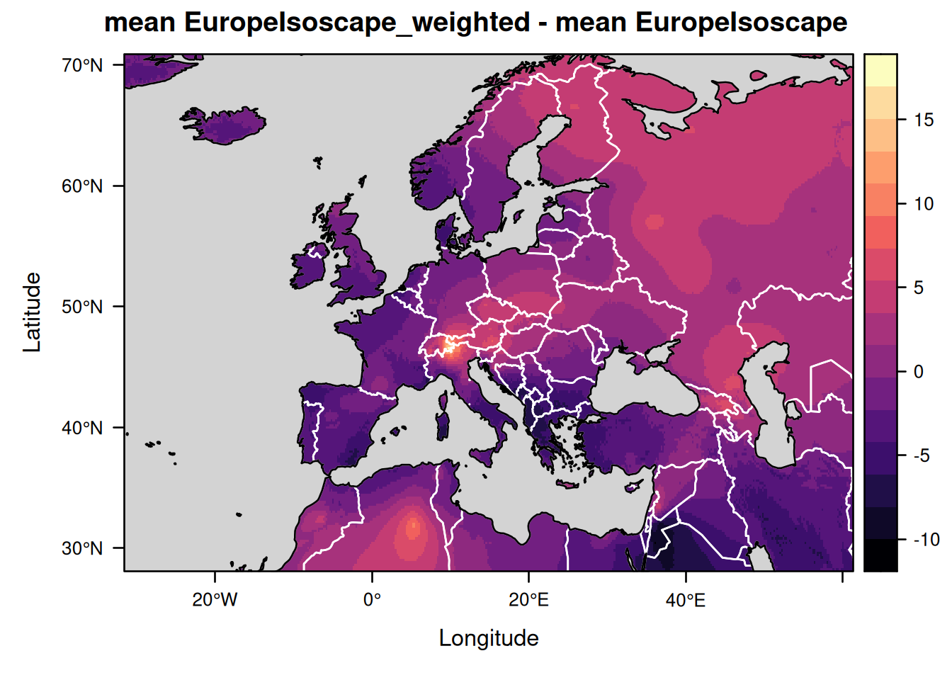
Let us similarly compare the isoscapes showing the prediction variance and the residual variance around the mean isoscape values:
levelplot(EuropeIsoscape_weighted$isoscapes$mean_predVar - EuropeIsoscape$isoscapes$mean_predVar,
          margin = FALSE,
          main = "predVar EuropeIsoscape_weighted - predVar EuropeIsoscape") +
  layer(lpolygon(CountryBorders, border = "white")) +
  layer(lpolygon(OceanMask, col = "lightgrey"))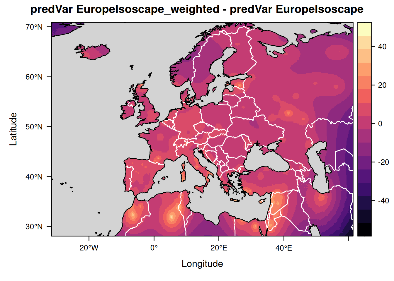
levelplot(EuropeIsoscape_weighted$isoscapes$mean_residVar - EuropeIsoscape$isoscapes$mean_residVar,
          margin = FALSE,
          main = "residVar EuropeIsoscape_weighted - residVar EuropeIsoscape") +
  layer(lpolygon(CountryBorders, border = "white")) +
  layer(lpolygon(OceanMask, col = "lightgrey"))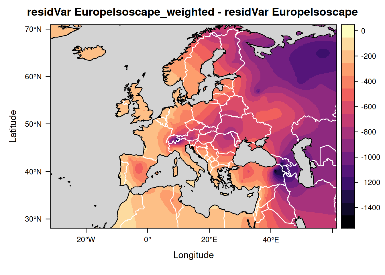
As you can see the residual variance is considerably smaller for the precipitation-weighted annual average isoscape than for the non-weighted isoscape. This is because the residual variance now represents the variation in isotopic values between years and no longer the total variation combining both the variations across years and months.
You could then continue with the calibration and assignment steps exactly as described in the chapters 4 & 5.
For this you simply need to replace the object EuropeIsoscape used in these chapters by the object EuropeIsoscape_weighted just created.