Chapter 4 Data manipulation with dplyr
dplyr is a package that makes data manipulation easy. It consists of five main verbs:
filter()arrange()select()mutate()summarise()
Other useful functions such as glimpse()
## Observations: 336,776
## Variables: 19
## $ year           <int> 2013, 2013, 2013, 2013, 2013, 2013, 2013, 2013, 2…
## $ month          <int> 1, 1, 1, 1, 1, 1, 1, 1, 1, 1, 1, 1, 1, 1, 1, 1, 1…
## $ day            <int> 1, 1, 1, 1, 1, 1, 1, 1, 1, 1, 1, 1, 1, 1, 1, 1, 1…
## $ dep_time       <int> 517, 533, 542, 544, 554, 554, 555, 557, 557, 558,…
## $ sched_dep_time <int> 515, 529, 540, 545, 600, 558, 600, 600, 600, 600,…
## $ dep_delay      <dbl> 2, 4, 2, -1, -6, -4, -5, -3, -3, -2, -2, -2, -2, …
## $ arr_time       <int> 830, 850, 923, 1004, 812, 740, 913, 709, 838, 753…
## $ sched_arr_time <int> 819, 830, 850, 1022, 837, 728, 854, 723, 846, 745…
## $ arr_delay      <dbl> 11, 20, 33, -18, -25, 12, 19, -14, -8, 8, -2, -3,…
## $ carrier        <chr> "UA", "UA", "AA", "B6", "DL", "UA", "B6", "EV", "…
## $ flight         <int> 1545, 1714, 1141, 725, 461, 1696, 507, 5708, 79, …
## $ tailnum        <chr> "N14228", "N24211", "N619AA", "N804JB", "N668DN",…
## $ origin         <chr> "EWR", "LGA", "JFK", "JFK", "LGA", "EWR", "EWR", …
## $ dest           <chr> "IAH", "IAH", "MIA", "BQN", "ATL", "ORD", "FLL", …
## $ air_time       <dbl> 227, 227, 160, 183, 116, 150, 158, 53, 140, 138, …
## $ distance       <dbl> 1400, 1416, 1089, 1576, 762, 719, 1065, 229, 944,…
## $ hour           <dbl> 5, 5, 5, 5, 6, 5, 6, 6, 6, 6, 6, 6, 6, 6, 6, 5, 6…
## $ minute         <dbl> 15, 29, 40, 45, 0, 58, 0, 0, 0, 0, 0, 0, 0, 0, 0,…
## $ time_hour      <dttm> 2013-01-01 05:00:00, 2013-01-01 05:00:00, 2013-0…
4.1 Excercise
- Import the customer data into R using
read_csv("path"), save it to a data.frame - Use
glimpse()on it
4.2 filter()
filter() is a function that let’s you filter out rows that meet certain conditions.
## # A tibble: 24,951 x 19
##     year month   day dep_time sched_dep_time dep_delay arr_time
##    <int> <int> <int>    <int>          <int>     <dbl>    <int>
##  1  2013     2     1      456            500        -4      652
##  2  2013     2     1      520            525        -5      816
##  3  2013     2     1      527            530        -3      837
##  4  2013     2     1      532            540        -8     1007
##  5  2013     2     1      540            540         0      859
##  6  2013     2     1      552            600        -8      714
##  7  2013     2     1      552            600        -8      919
##  8  2013     2     1      552            600        -8      655
##  9  2013     2     1      553            600        -7      833
## 10  2013     2     1      553            600        -7      821
## # … with 24,941 more rows, and 12 more variables: sched_arr_time <int>,
## #   arr_delay <dbl>, carrier <chr>, flight <int>, tailnum <chr>,
## #   origin <chr>, dest <chr>, air_time <dbl>, distance <dbl>, hour <dbl>,
## #   minute <dbl>, time_hour <dttm>
We can also use text:
## # A tibble: 111,279 x 19
##     year month   day dep_time sched_dep_time dep_delay arr_time
##    <int> <int> <int>    <int>          <int>     <dbl>    <int>
##  1  2013     1     1      542            540         2      923
##  2  2013     1     1      544            545        -1     1004
##  3  2013     1     1      557            600        -3      838
##  4  2013     1     1      558            600        -2      849
##  5  2013     1     1      558            600        -2      853
##  6  2013     1     1      558            600        -2      924
##  7  2013     1     1      559            559         0      702
##  8  2013     1     1      606            610        -4      837
##  9  2013     1     1      611            600        11      945
## 10  2013     1     1      613            610         3      925
## # … with 111,269 more rows, and 12 more variables: sched_arr_time <int>,
## #   arr_delay <dbl>, carrier <chr>, flight <int>, tailnum <chr>,
## #   origin <chr>, dest <chr>, air_time <dbl>, distance <dbl>, hour <dbl>,
## #   minute <dbl>, time_hour <dttm>
And combine them:
## # A tibble: 8,421 x 19
##     year month   day dep_time sched_dep_time dep_delay arr_time
##    <int> <int> <int>    <int>          <int>     <dbl>    <int>
##  1  2013     2     1      532            540        -8     1007
##  2  2013     2     1      540            540         0      859
##  3  2013     2     1      552            600        -8      714
##  4  2013     2     1      554            601        -7      920
##  5  2013     2     1      555            600        -5      903
##  6  2013     2     1      558            600        -2      916
##  7  2013     2     1      559            600        -1      923
##  8  2013     2     1      602            600         2      655
##  9  2013     2     1      609            610        -1      902
## 10  2013     2     1      610            615        -5      905
## # … with 8,411 more rows, and 12 more variables: sched_arr_time <int>,
## #   arr_delay <dbl>, carrier <chr>, flight <int>, tailnum <chr>,
## #   origin <chr>, dest <chr>, air_time <dbl>, distance <dbl>, hour <dbl>,
## #   minute <dbl>, time_hour <dttm>
We can also filter out every row that meets a condition in a vector, for instance:
## # A tibble: 215,941 x 19
##     year month   day dep_time sched_dep_time dep_delay arr_time
##    <int> <int> <int>    <int>          <int>     <dbl>    <int>
##  1  2013     1     1      533            529         4      850
##  2  2013     1     1      542            540         2      923
##  3  2013     1     1      544            545        -1     1004
##  4  2013     1     1      554            600        -6      812
##  5  2013     1     1      557            600        -3      709
##  6  2013     1     1      557            600        -3      838
##  7  2013     1     1      558            600        -2      753
##  8  2013     1     1      558            600        -2      849
##  9  2013     1     1      558            600        -2      853
## 10  2013     1     1      558            600        -2      924
## # … with 215,931 more rows, and 12 more variables: sched_arr_time <int>,
## #   arr_delay <dbl>, carrier <chr>, flight <int>, tailnum <chr>,
## #   origin <chr>, dest <chr>, air_time <dbl>, distance <dbl>, hour <dbl>,
## #   minute <dbl>, time_hour <dttm>
4.2.1 Operators
In R, as in any programming languange, there are a number of logical and relational operators.
In R these are:
## # A tibble: 3 x 2
##   `Relation operators` `Symbol in R`
##   <chr>                <chr>
## 1 "och (and) "         &
## 2 eller(or)            |
## 3 icke(not)            !
## # A tibble: 7 x 2
## `Logical Operators` `Symbol in R`
## <chr> <chr>
## 1 equal ==
## 2 not equal !=
## 3 larger than or equal >=
## 4 smaller than or equal <=
## 5 larger than >
## 6 smaller than <
## 7 is in %in%4.3 We also have operators for checking if something is TRUE
- Instead of writing
x == TRUEyou should writeisTRUE(x)and!isTRUE(x)if you want to check if something isFALSE.
4.3.1 Use filter to find…
How many customers had a data-volume over 1000 in february 2019?
How many customers have been members longer than 2005
How many customers have a data-volume over 2000 in february and have a calculated revenue larger than 500 per month?
How many customers have a subscription with “Rörlig pris”?
Are there any customers that are missing an ID? I.e. is
NA.
4.3.2 stringr
- When working
filter()it is common that we want to filter out certains parts of a string stringris a great package for manipulating strings in R- Usually it’s functions starts with
str_..., such asstr_detect().
Here are some useful functions:
## [1] FALSE FALSE TRUEOr str_replace()
## [1] "äpple" "oränge" "bänana"Or str_remove()
## [1] "pple" "ornge" "bnana"4.3.3 stringr in filter()
We can use stringr in filter():
## # A tibble: 79,201 x 19
##     year month   day dep_time sched_dep_time dep_delay arr_time
##    <int> <int> <int>    <int>          <int>     <dbl>    <int>
##  1  2013     1     1      517            515         2      830
##  2  2013     1     1      533            529         4      850
##  3  2013     1     1      554            558        -4      740
##  4  2013     1     1      558            600        -2      924
##  5  2013     1     1      558            600        -2      923
##  6  2013     1     1      559            600        -1      854
##  7  2013     1     1      607            607         0      858
##  8  2013     1     1      611            600        11      945
##  9  2013     1     1      622            630        -8     1017
## 10  2013     1     1      623            627        -4      933
## # … with 79,191 more rows, and 12 more variables: sched_arr_time <int>,
## #   arr_delay <dbl>, carrier <chr>, flight <int>, tailnum <chr>,
## #   origin <chr>, dest <chr>, air_time <dbl>, distance <dbl>, hour <dbl>,
## #   minute <dbl>, time_hour <dttm>
4.4 Regex
- Specific string manipulation
For example:
## [1] "apple" "orange" "banana"## [1] FALSE FALSE TRUEand
## [1] "apple" "orange" "banana"## [1] TRUE TRUE FALSE4.5 Excercise 2
- How many customers have a subscription with “Fast pris”?
- How many customers have a subscription that is not “Bredband”?
4.6 arrange()
arrange() is a verb for sorting data.frames.
## # A tibble: 336,776 x 19
##     year month   day dep_time sched_dep_time dep_delay arr_time
##    <int> <int> <int>    <int>          <int>     <dbl>    <int>
##  1  2013    12     7     2040           2123       -43       40
##  2  2013     2     3     2022           2055       -33     2240
##  3  2013    11    10     1408           1440       -32     1549
##  4  2013     1    11     1900           1930       -30     2233
##  5  2013     1    29     1703           1730       -27     1947
##  6  2013     8     9      729            755       -26     1002
##  7  2013    10    23     1907           1932       -25     2143
##  8  2013     3    30     2030           2055       -25     2213
##  9  2013     3     2     1431           1455       -24     1601
## 10  2013     5     5      934            958       -24     1225
## # … with 336,766 more rows, and 12 more variables: sched_arr_time <int>,
## #   arr_delay <dbl>, carrier <chr>, flight <int>, tailnum <chr>,
## #   origin <chr>, dest <chr>, air_time <dbl>, distance <dbl>, hour <dbl>,
## #   minute <dbl>, time_hour <dttm>
If you instead want to sort in descending order you can write like this:
## # A tibble: 336,776 x 19
##     year month   day dep_time sched_dep_time dep_delay arr_time
##    <int> <int> <int>    <int>          <int>     <dbl>    <int>
##  1  2013     1     9      641            900      1301     1242
##  2  2013     6    15     1432           1935      1137     1607
##  3  2013     1    10     1121           1635      1126     1239
##  4  2013     9    20     1139           1845      1014     1457
##  5  2013     7    22      845           1600      1005     1044
##  6  2013     4    10     1100           1900       960     1342
##  7  2013     3    17     2321            810       911      135
##  8  2013     6    27      959           1900       899     1236
##  9  2013     7    22     2257            759       898      121
## 10  2013    12     5      756           1700       896     1058
## # … with 336,766 more rows, and 12 more variables: sched_arr_time <int>,
## #   arr_delay <dbl>, carrier <chr>, flight <int>, tailnum <chr>,
## #   origin <chr>, dest <chr>, air_time <dbl>, distance <dbl>, hour <dbl>,
## #   minute <dbl>, time_hour <dttm>
4.6.0.1 Excercise 3
- Which customer has been “active” longest? What is the date?
- Which customer is most newly active?
4.7 select()
select() is a verb for selecting columns in a data.frame.
You can choose columns by their name:
## # A tibble: 336,776 x 4
##     year month   day origin
##    <int> <int> <int> <chr>
##  1  2013     1     1 EWR
##  2  2013     1     1 LGA
##  3  2013     1     1 JFK
##  4  2013     1     1 JFK
##  5  2013     1     1 LGA
##  6  2013     1     1 EWR
##  7  2013     1     1 EWR
##  8  2013     1     1 LGA
##  9  2013     1     1 JFK
## 10  2013     1     1 LGA
## # … with 336,766 more rows
You can also choose columns based on their numerical order
## # A tibble: 336,776 x 5
##     year month   day dep_time sched_dep_time
##    <int> <int> <int>    <int>          <int>
##  1  2013     1     1      517            515
##  2  2013     1     1      533            529
##  3  2013     1     1      542            540
##  4  2013     1     1      544            545
##  5  2013     1     1      554            600
##  6  2013     1     1      554            558
##  7  2013     1     1      555            600
##  8  2013     1     1      557            600
##  9  2013     1     1      557            600
## 10  2013     1     1      558            600
## # … with 336,766 more rows
You can select all the columns from column_a to column_d with: :
## # A tibble: 336,776 x 13
##     year month   day dep_time sched_dep_time dep_delay arr_time
##    <int> <int> <int>    <int>          <int>     <dbl>    <int>
##  1  2013     1     1      517            515         2      830
##  2  2013     1     1      533            529         4      850
##  3  2013     1     1      542            540         2      923
##  4  2013     1     1      544            545        -1     1004
##  5  2013     1     1      554            600        -6      812
##  6  2013     1     1      554            558        -4      740
##  7  2013     1     1      555            600        -5      913
##  8  2013     1     1      557            600        -3      709
##  9  2013     1     1      557            600        -3      838
## 10  2013     1     1      558            600        -2      753
## # … with 336,766 more rows, and 6 more variables: sched_arr_time <int>,
## #   arr_delay <dbl>, carrier <chr>, flight <int>, tailnum <chr>,
## #   origin <chr>
4.7.1 Help functions
When you do data science you often want to move columns for different reasons. Not seldom you want to put one column first and the rest after. For this you can use the help function everything():
## # A tibble: 336,776 x 19
##    origin  year month   day dep_time sched_dep_time dep_delay arr_time
##    <chr>  <int> <int> <int>    <int>          <int>     <dbl>    <int>
##  1 EWR     2013     1     1      517            515         2      830
##  2 LGA     2013     1     1      533            529         4      850
##  3 JFK     2013     1     1      542            540         2      923
##  4 JFK     2013     1     1      544            545        -1     1004
##  5 LGA     2013     1     1      554            600        -6      812
##  6 EWR     2013     1     1      554            558        -4      740
##  7 EWR     2013     1     1      555            600        -5      913
##  8 LGA     2013     1     1      557            600        -3      709
##  9 JFK     2013     1     1      557            600        -3      838
## 10 LGA     2013     1     1      558            600        -2      753
## # … with 336,766 more rows, and 11 more variables: sched_arr_time <int>,
## #   arr_delay <dbl>, carrier <chr>, flight <int>, tailnum <chr>,
## #   dest <chr>, air_time <dbl>, distance <dbl>, hour <dbl>, minute <dbl>,
## #   time_hour <dttm>
Apart from eveything() there are a number of other help functions:
starts_with(“asd”)
ends_with(“air”)
contains(“flyg”)
matches(“asd”)
num_range(“flyg”, 1:10) matches flyg1, flyg2 … flyg10
You can use these in the same way as everything().
## # A tibble: 336,776 x 3
##    origin month minute
##    <chr>  <int>  <dbl>
##  1 EWR        1     15
##  2 LGA        1     29
##  3 JFK        1     40
##  4 JFK        1     45
##  5 LGA        1      0
##  6 EWR        1     58
##  7 EWR        1      0
##  8 LGA        1      0
##  9 JFK        1      0
## 10 LGA        1      0
## # … with 336,766 more rows
4.8 rename()
To rename a variable you use rename(data, new_variable = old_variable)
## # A tibble: 336,776 x 19
##       år month   day dep_time sched_dep_time dep_delay arr_time
##    <int> <int> <int>    <int>          <int>     <dbl>    <int>
##  1  2013     1     1      517            515         2      830
##  2  2013     1     1      533            529         4      850
##  3  2013     1     1      542            540         2      923
##  4  2013     1     1      544            545        -1     1004
##  5  2013     1     1      554            600        -6      812
##  6  2013     1     1      554            558        -4      740
##  7  2013     1     1      555            600        -5      913
##  8  2013     1     1      557            600        -3      709
##  9  2013     1     1      557            600        -3      838
## 10  2013     1     1      558            600        -2      753
## # … with 336,766 more rows, and 12 more variables: sched_arr_time <int>,
## #   arr_delay <dbl>, carrier <chr>, flight <int>, tailnum <chr>,
## #   origin <chr>, dest <chr>, air_time <dbl>, distance <dbl>, hour <dbl>,
## #   minute <dbl>, time_hour <dttm>
4.9 Excercise 4
Choose all columns that contain ”nm"
Choose the column for customer ID and all columns that starts with ”tr_tot"
Rename ”pc_priceplan_nm" to ”price_plan"
4.10 mutate()
mutate()is a verb for manipulating and creating new columns
Below we create a new column with the mean of departure delay.
## # A tibble: 336,776 x 20
##     year month   day dep_time sched_dep_time dep_delay arr_time
##    <int> <int> <int>    <int>          <int>     <dbl>    <int>
##  1  2013     1     1      517            515         2      830
##  2  2013     1     1      533            529         4      850
##  3  2013     1     1      542            540         2      923
##  4  2013     1     1      544            545        -1     1004
##  5  2013     1     1      554            600        -6      812
##  6  2013     1     1      554            558        -4      740
##  7  2013     1     1      555            600        -5      913
##  8  2013     1     1      557            600        -3      709
##  9  2013     1     1      557            600        -3      838
## 10  2013     1     1      558            600        -2      753
## # … with 336,766 more rows, and 13 more variables: sched_arr_time <int>,
## #   arr_delay <dbl>, carrier <chr>, flight <int>, tailnum <chr>,
## #   origin <chr>, dest <chr>, air_time <dbl>, distance <dbl>, hour <dbl>,
## #   minute <dbl>, time_hour <dttm>, mean_dep_delay <dbl>
You can also use with simple mathematical operators mutate():
## # A tibble: 336,776 x 20
##     year month   day dep_time sched_dep_time dep_delay arr_time
##    <int> <int> <int>    <int>          <int>     <dbl>    <int>
##  1  2013     1     1      517            515         2      830
##  2  2013     1     1      533            529         4      850
##  3  2013     1     1      542            540         2      923
##  4  2013     1     1      544            545        -1     1004
##  5  2013     1     1      554            600        -6      812
##  6  2013     1     1      554            558        -4      740
##  7  2013     1     1      555            600        -5      913
##  8  2013     1     1      557            600        -3      709
##  9  2013     1     1      557            600        -3      838
## 10  2013     1     1      558            600        -2      753
## # … with 336,766 more rows, and 13 more variables: sched_arr_time <int>,
## #   arr_delay <dbl>, carrier <chr>, flight <int>, tailnum <chr>,
## #   origin <chr>, dest <chr>, air_time <dbl>, distance <dbl>, hour <dbl>,
## #   minute <dbl>, time_hour <dttm>, beer_time <dbl>
There is a variant of mutate mutate() calledtransmute() that will return only the column that you have maniuplated.
## # A tibble: 336,776 x 1
##    beer_time
##        <dbl>
##  1        -9
##  2       -16
##  3       -31
##  4        17
##  5        19
##  6       -16
##  7       -24
##  8        11
##  9         5
## 10       -10
## # … with 336,766 more rows
In combination with mutate() you can use a variety of functions, some example of useful functions inside mutate is:
rank(), min_rank(), dense_rank(), percent_rank() to rank
log(), log10() to take the log of a variable
cumsum(), cummean() for cummulative stats
row_number() if you need to create rownumbers
lead() and lag()
For example we can lag departure delay and save it in a new variable.
## # A tibble: 336,776 x 1
##    lag_dep_delay
##            <dbl>
##  1            NA
##  2             2
##  3             4
##  4             2
##  5            -1
##  6            -6
##  7            -4
##  8            -5
##  9            -3
## 10            -3
## # … with 336,766 more rows
4.10.1 if_else()
- A common task in Excel or any other programming languange is to compose
if else-statements. - The best way to do this in R is with the function
if_else()
## # A tibble: 336,776 x 1
##    försenad
##    <chr>
##  1 ej försenad
##  2 ej försenad
##  3 ej försenad
##  4 ej försenad
##  5 ej försenad
##  6 ej försenad
##  7 ej försenad
##  8 ej försenad
##  9 ej försenad
## 10 ej försenad
## # … with 336,766 more rows
If you want to make multiple if else-statements, instead of making multiple if else-statements you can use the case_when() function:
transmute(flights, försenad_kat = case_when(
  dep_delay + arr_delay > 80 ~ "mycket_försenad",
  dep_delay + arr_delay > 0 ~ "ganska_försenad",
  dep_delay + arr_delay  <= 0 ~ "ej_försenad",
  TRUE ~ "okänd"))
## # A tibble: 336,776 x 1
## försenad_kat
## <chr>
## 1 ganska_försenad
## 2 ganska_försenad
## 3 ganska_försenad
## 4 ej_försenad
## 5 ej_försenad
## 6 ganska_försenad
## 7 ganska_försenad
## 8 ej_försenad
## 9 ej_försenad
## 10 ganska_försenad
## # … with 336,766 more rows4.11 Excercise 5
Create a new variable that is the mean of the last 3 months of data consumption
Create a variable that takes the logarithm of your previously created column
Create a new variable that indicates if the priceplan is “Bredband” or not.
Create a new variable that groups priceplan in “Fast pris”, “Rörligt pris”, “Bredband” and “Annan” for everything that is not in any of the previous.
4.12 Dates
- Dates a information about time that we commonly use in analytics.
- The easiest way to manipulate dates in R is with the package
lubridate.
In order to get todays date you can use the function Sys.Date()(that is built into R).
## [1] "2019-09-17"Say that you want to find the month, week or year of a date.
The package lubridate contains useful functions for this, such as year(), month() and week.
##
## Attaching package: 'lubridate'
## The following object is masked from 'package:base':
##
## date## [1] 38In general you should define your date before passing it to a lubridate-function. In other words, you can’t just use a string (even though that sometimes work).
## Error in leap_year(x): unrecognized date formatYou can define you with with as.Date(), where you also can specify the format of the date.
## [1] "2018-03-15"This is especially useful if your date is written in a non-standard way.
## [1] "2018-03-15"Other functions that are useful in lubridate are days_in_month:
## Mar
##  31
And floor_date() if you, for example, want to find the first date in a month or a week,.
## [1] "2018-03-01"4.13 Excercise 6
- Create a varible for month
lubridate::month(x)of customer activation - Create a new varibale for
yearof customer activation - Create a new variable with the number of days in the month of activation
4.14 summarise()
summarise() is a verb for summarizing data (you can also spell i summarize()).
summarise(flights,
          mean_dist = mean(distance, na.rm = T),
          median_dist = median(distance, na.rm = T),
          sum_dist = sum(distance, na.rm = T)
)
## # A tibble: 1 x 3
## mean_dist median_dist sum_dist
## <dbl> <dbl> <dbl>
## 1 1040. 872 3502176074.14.1 group_by()
Below we create a new grouped data set grouped on carrier och dest.
Every summarisation or mutation done on this new data-set will be done group wise.
## # A tibble: 314 x 3
## # Groups:   carrier [16]
##    carrier dest  mean_dep_delay
##    <chr>   <chr>          <dbl>
##  1 9E      ATL            0.965
##  2 9E      AUS           19
##  3 9E      AVL           -2.6
##  4 9E      BGR           34
##  5 9E      BNA           19.1
##  6 9E      BOS           14.8
##  7 9E      BTV           -4.5
##  8 9E      BUF           15.5
##  9 9E      BWI           17.5
## 10 9E      CAE           -3.67
## # … with 304 more rows
4.15 Excercise 7
- What is the sum data volume during the last month? What’s the mean and median and what are the max and min values? You can use
max()andmin()to calculate maximum and minimum-values.
4.15.1 More expressions
You can combine dplyr-verbs
## # A tibble: 16 x 2
##    carrier mean_dep_delay
##    <chr>            <dbl>
##  1 9E               16.7
##  2 AA                8.59
##  3 AS                5.80
##  4 B6               13.0
##  5 DL                9.26
##  6 EV               20.0
##  7 F9               20.2
##  8 FL               18.7
##  9 HA                4.90
## 10 MQ               10.6
## 11 OO               12.6
## 12 UA               12.1
## 13 US                3.78
## 14 VX               12.9
## 15 WN               17.7
## 16 YV               19.0
However, the more verbs you combine the harder it will be to read:
summarise(
  group_by(
    filter(flights, dep_delay < 60),
    carrier),
  mean_dep_delay = mean(dep_delay, na.rm = T), n_flights = n())
## # A tibble: 16 x 3
## carrier mean_dep_delay n_flights
## <chr> <dbl> <int>
## 1 9E 2.96 15425
## 2 AA 0.890 30059
## 3 AS -0.719 673
## 4 B6 3.26 49514
## 5 DL 1.76 45062
## 6 EV 4.65 44372
## 7 F9 5.09 607
## 8 FL 4.72 2864
## 9 HA -2.47 331
## 10 MQ 1.48 23126
## 11 OO -2.88 25
## 12 UA 4.33 54080
## 13 US -0.744 19094
## 14 VX 2.70 4766
## 15 WN 6.60 10999
## 16 YV 2.25 4654.15.1.1 %>% “the pipe”
%>%from themagrittr-package.%>%is called “the pipe” and is pronounced “and then”.
flights %>%
  filter(dep_delay < 60) %>%
  group_by(carrier) %>%
  summarise(
    mean_dep_delay = mean(dep_delay, na.rm = T),
    n_flights = n()
  )
## # A tibble: 16 x 3
## carrier mean_dep_delay n_flights
## <chr> <dbl> <int>
## 1 9E 2.96 15425
## 2 AA 0.890 30059
## 3 AS -0.719 673
## 4 B6 3.26 49514
## 5 DL 1.76 45062
## 6 EV 4.65 44372
## 7 F9 5.09 607
## 8 FL 4.72 2864
## 9 HA -2.47 331
## 10 MQ 1.48 23126
## 11 OO -2.88 25
## 12 UA 4.33 54080
## 13 US -0.744 19094
## 14 VX 2.70 4766
## 15 WN 6.60 10999
## 16 YV 2.25 4654.16 Excercise 8
Use %>% and answer the following questions:
Which CPE type is most common?
Which priceplan has the highest mean data volume (for febraury 2019)?
Calculate the mean of data volume for the year that the customer was created. Which year has the highest mean?
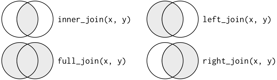
4.17 Joins
To join data frames is an essential part of data manipulation, to do that we use dplyr’s different join functions:
left_join()right_join()full_join()inner_join()semi_join()anti_join()
4.18 Joins som venn
flights %>%
  select(year:day, hour, origin, dest, tailnum, carrier) %>%
  left_join(airlines, by = c("carrier" = "carrier"))
## # A tibble: 336,776 x 9
## year month day hour origin dest tailnum carrier name
## <int> <int> <int> <dbl> <chr> <chr> <chr> <chr> <chr>
## 1 2013 1 1 5 EWR IAH N14228 UA United Air Lines I…
## 2 2013 1 1 5 LGA IAH N24211 UA United Air Lines I…
## 3 2013 1 1 5 JFK MIA N619AA AA American Airlines …
## 4 2013 1 1 5 JFK BQN N804JB B6 JetBlue Airways
## 5 2013 1 1 6 LGA ATL N668DN DL Delta Air Lines In…
## 6 2013 1 1 5 EWR ORD N39463 UA United Air Lines I…
## 7 2013 1 1 6 EWR FLL N516JB B6 JetBlue Airways
## 8 2013 1 1 6 LGA IAD N829AS EV ExpressJet Airline…
## 9 2013 1 1 6 JFK MCO N593JB B6 JetBlue Airways
## 10 2013 1 1 6 LGA ORD N3ALAA AA American Airlines …
## # … with 336,766 more rows4.19 Excercise 9
- Left join your data with
tele2-kunder-transaktioner.csvoncustid.
4.20 Tidy data
tidydata is when every observation is a row and every variable is a column.
## # A tibble: 1,704 x 6
##    country     continent  year lifeExp      pop gdpPercap
##    <fct>       <fct>     <int>   <dbl>    <int>     <dbl>
##  1 Afghanistan Asia       1952    28.8  8425333      779.
##  2 Afghanistan Asia       1957    30.3  9240934      821.
##  3 Afghanistan Asia       1962    32.0 10267083      853.
##  4 Afghanistan Asia       1967    34.0 11537966      836.
##  5 Afghanistan Asia       1972    36.1 13079460      740.
##  6 Afghanistan Asia       1977    38.4 14880372      786.
##  7 Afghanistan Asia       1982    39.9 12881816      978.
##  8 Afghanistan Asia       1987    40.8 13867957      852.
##  9 Afghanistan Asia       1992    41.7 16317921      649.
## 10 Afghanistan Asia       1997    41.8 22227415      635.
## # … with 1,694 more rows
4.21 Untidy data
library(readxl)
gapminder_untidy <- read_excel("data/life_expectancy_at_birth.xlsx")
gapminder_untidy
## # A tibble: 260 x 218
## `Life expectanc… `1800` `1801` `1802` `1803` `1804` `1805` `1806` `1807`
## <chr> <dbl> <dbl> <dbl> <dbl> <dbl> <dbl> <dbl> <dbl>
## 1 Abkhazia NA NA NA NA NA NA NA NA
## 2 Afghanistan 28.2 28.2 28.2 28.2 28.2 28.2 28.2 28.1
## 3 Akrotiri and Dh… NA NA NA NA NA NA NA NA
## 4 Albania 35.4 35.4 35.4 35.4 35.4 35.4 35.4 35.4
## 5 Algeria 28.8 28.8 28.8 28.8 28.8 28.8 28.8 28.8
## 6 American Samoa NA NA NA NA NA NA NA NA
## 7 Andorra NA NA NA NA NA NA NA NA
## 8 Angola 27.0 27.0 27.0 27.0 27.0 27.0 27.0 27.0
## 9 Anguilla NA NA NA NA NA NA NA NA
## 10 Antigua and Bar… 33.5 33.5 33.5 33.5 33.5 33.5 33.5 33.5
## # … with 250 more rows, and 209 more variables: `1808` <dbl>,
## # `1809` <dbl>, `1810` <dbl>, `1811` <dbl>, `1812` <dbl>, `1813` <dbl>,
## # `1814` <dbl>, `1815` <dbl>, `1816` <dbl>, `1817` <dbl>, `1818` <dbl>,
## # `1819` <dbl>, `1820` <dbl>, `1821` <dbl>, `1822` <dbl>, `1823` <dbl>,
## # `1824` <dbl>, `1825` <dbl>, `1826` <dbl>, `1827` <dbl>, `1828` <dbl>,
## # `1829` <dbl>, `1830` <dbl>, `1831` <dbl>, `1832` <dbl>, `1833` <dbl>,
## # `1834` <dbl>, `1835` <dbl>, `1836` <dbl>, `1837` <dbl>, `1838` <dbl>,
## # `1839` <dbl>, `1840` <dbl>, `1841` <dbl>, `1842` <dbl>, `1843` <dbl>,
## # `1844` <dbl>, `1845` <dbl>, `1846` <dbl>, `1847` <dbl>, `1848` <dbl>,
## # `1849` <dbl>, `1850` <dbl>, `1851` <dbl>, `1852` <dbl>, `1853` <dbl>,
## # `1854` <dbl>, `1855` <dbl>, `1856` <dbl>, `1857` <dbl>, `1858` <dbl>,
## # `1859` <dbl>, `1860` <dbl>, `1861` <dbl>, `1862` <dbl>, `1863` <dbl>,
## # `1864` <dbl>, `1865` <dbl>, `1866` <dbl>, `1867` <dbl>, `1868` <dbl>,
## # `1869` <dbl>, `1870` <dbl>, `1871` <dbl>, `1872` <dbl>, `1873` <dbl>,
## # `1874` <dbl>, `1875` <dbl>, `1876` <dbl>, `1877` <dbl>, `1878` <dbl>,
## # `1879` <dbl>, `1880` <dbl>, `1881` <dbl>, `1882` <dbl>, `1883` <dbl>,
## # `1884` <dbl>, `1885` <dbl>, `1886` <dbl>, `1887` <dbl>, `1888` <dbl>,
## # `1889` <dbl>, `1890` <dbl>, `1891` <dbl>, `1892` <dbl>, `1893` <dbl>,
## # `1894` <dbl>, `1895` <dbl>, `1896` <dbl>, `1897` <dbl>, `1898` <dbl>,
## # `1899` <dbl>, `1900` <dbl>, `1901` <dbl>, `1902` <dbl>, `1903` <dbl>,
## # `1904` <dbl>, `1905` <dbl>, `1906` <dbl>, `1907` <dbl>, …We want to gather the columns
gapminder_untidy %>%
  gather(key = year, value = life_expectancy, -`Life expectancy`) %>%
  rename(land = `Life expectancy`) %>%
  mutate(life_expectancy = as.numeric(life_expectancy))
## # A tibble: 56,420 x 3
## land year life_expectancy
## <chr> <chr> <dbl>
## 1 Abkhazia 1800 NA
## 2 Afghanistan 1800 28.2
## 3 Akrotiri and Dhekelia 1800 NA
## 4 Albania 1800 35.4
## 5 Algeria 1800 28.8
## 6 American Samoa 1800 NA
## 7 Andorra 1800 NA
## 8 Angola 1800 27.0
## 9 Anguilla 1800 NA
## 10 Antigua and Barbuda 1800 33.5
## # … with 56,410 more rowsspread()does the opposite.
4.22 Excercise 10
In your data set you have 12 columns for data volume consumption per month,
tr_tot_data_vol_all_netw_1:tr_tot_data_vol_all_netw_12Every column represent a month and you want to calculate the mean of data volume consumption over time.
The columns represent a month
The first column
tr_tot_data_vol_all_netw_1is the latest month, i.e. “2019-04-30”Create a vector with all the month dates corresponding to the columns.
R function called
seq()
new_cols <- seq(from = as.Date("2018-05-30"), by = "month", length.out = 12) %>%
  as.character()

new_cols
## [1] "2018-05-30" "2018-06-30" "2018-07-30" "2018-08-30" "2018-09-30"
## [6] "2018-10-30" "2018-11-30" "2018-12-30" "2019-01-30" "2019-03-02"
## [11] "2019-03-30" "2019-04-30"Rename every column by it’s date.
kunder %>%
  select(cust_id, source_date, pc_priceplan_nm, tr_tot_data_vol_all_netw_1:tr_tot_data_vol_all_netw_12) %>%
rename_at(vars(tr_tot_data_vol_all_netw_1:tr_tot_data_vol_all_netw_12), ~new_cols)- Fill in the
sort(decreasing = )toTRUE - Gather the data into two new columns called
data_monthanddata_volume - Turn
data_monthinto a date-column
new_cols <- seq(from = as.Date("2018-05-30"), by = "month", length.out = 12) %>%
  sort(decreasing = ) %>%
  as.character()

kunder_tidy_month <- kunder %>%
  select(cust_id, source_date, pc_priceplan_nm, tr_tot_data_vol_all_netw_1:tr_tot_data_vol_all_netw_12) %>%
  rename_at(vars(tr_tot_data_vol_all_netw_1:tr_tot_data_vol_all_netw_12), ~new_cols) %>%
  gather(... , ... , `2018-05-30`:`2019-04-30`) %>%
mutate(data_month = as.Date(data_month))- Calculate the mean value per priceplan and month
mean_volume_sum <- kunder_tidy_month %>%
  group_by(pc_priceplan_nm, data_month) %>%
  summarise(mean_volume = mean(data_volume, na.rm = T))

mean_volume_sum
Execute the code to visualize:
p <- ggplot(mean_volume_sum,
         aes(x = data_month, y = mean_volume, color = pc_priceplan_nm)) +
  geom_line() +
  scale_color_discrete() +
theme(legend.position = "none")<iframe src=“plotly_ex.html” width = “900px”, height = “600px” frameBorder=“0”>