Chapter 7 Advanced data manipulation

7.1 Agenda

• Base R
• Functions
• Iterations
• Advanced dplyr

7.2 Functions

We know functions from before:

• mean()

7.3 Functions are automation

• generate_report()
• train_model()
• write_xlsx_tables()
• create_ppt()

7.4 When should we write a function?

The automation rule

• Consider writing a function whenever you’ve copied and pasted a block of code more than twice.

7.5 Introduction to base R

• The native languange of R
• dplyr or other packages are dialects

7.5.1 selecting cols

With dplyr:

library(dplyr)

cars_select <- select(.data = mtcars, hp, mpg, qsec)

With base R - Brackets [] on data.frame

cars_select <- mtcars[rows, columns]

cars_select <- mtcars[, c("hp", "mpg", "qsec")]

7.5.2 Filter and select

mtcars %>% 
    select(hp, mpg, qsec) %>% 
    filter(hp > 100)

##     hp  mpg  qsec
## 1  110 21.0 16.46
## 2  110 21.0 17.02
## 3  110 21.4 19.44
## 4  175 18.7 17.02
## 5  105 18.1 20.22
## 6  245 14.3 15.84
## 7  123 19.2 18.30
## 8  123 17.8 18.90
## 9  180 16.4 17.40
## 10 180 17.3 17.60
## 11 180 15.2 18.00
## 12 205 10.4 17.98
## 13 215 10.4 17.82
## 14 230 14.7 17.42
## 15 150 15.5 16.87
## 16 150 15.2 17.30
## 17 245 13.3 15.41
## 18 175 19.2 17.05
## 19 113 30.4 16.90
## 20 264 15.8 14.50
## 21 175 19.7 15.50
## 22 335 15.0 14.60
## 23 109 21.4 18.60

With base R

mtcars[mtcars$hp > 100, c("hp", "mpg", "qsec")]

##                      hp  mpg  qsec
## Mazda RX4           110 21.0 16.46
## Mazda RX4 Wag       110 21.0 17.02
## Hornet 4 Drive      110 21.4 19.44
## Hornet Sportabout   175 18.7 17.02
## Valiant             105 18.1 20.22
## Duster 360          245 14.3 15.84
## Merc 280            123 19.2 18.30
## Merc 280C           123 17.8 18.90
## Merc 450SE          180 16.4 17.40
## Merc 450SL          180 17.3 17.60
## Merc 450SLC         180 15.2 18.00
## Cadillac Fleetwood  205 10.4 17.98
## Lincoln Continental 215 10.4 17.82
## Chrysler Imperial   230 14.7 17.42
## Dodge Challenger    150 15.5 16.87
## AMC Javelin         150 15.2 17.30
## Camaro Z28          245 13.3 15.41
## Pontiac Firebird    175 19.2 17.05
## Lotus Europa        113 30.4 16.90
## Ford Pantera L      264 15.8 14.50
## Ferrari Dino        175 19.7 15.50
## Maserati Bora       335 15.0 14.60
## Volvo 142E          109 21.4 18.60

7.6 The syntax of package data.table

library(data.table)

## 
## Attaching package: 'data.table'

## The following objects are masked from 'package:lubridate':
## 
##     hour, isoweek, mday, minute, month, quarter, second, wday,
##     week, yday, year

## The following objects are masked from 'package:dplyr':
## 
##     between, first, last

## The following object is masked from 'package:purrr':
## 
##     transpose

mtcars <- as.data.table(mtcars)

mtcars[hp > 100, .(hp, mpg, qsec)]

##      hp  mpg  qsec
##  1: 110 21.0 16.46
##  2: 110 21.0 17.02
##  3: 110 21.4 19.44
##  4: 175 18.7 17.02
##  5: 105 18.1 20.22
##  6: 245 14.3 15.84
##  7: 123 19.2 18.30
##  8: 123 17.8 18.90
##  9: 180 16.4 17.40
## 10: 180 17.3 17.60
## 11: 180 15.2 18.00
## 12: 205 10.4 17.98
## 13: 215 10.4 17.82
## 14: 230 14.7 17.42
## 15: 150 15.5 16.87
## 16: 150 15.2 17.30
## 17: 245 13.3 15.41
## 18: 175 19.2 17.05
## 19: 113 30.4 16.90
## 20: 264 15.8 14.50
## 21: 175 19.7 15.50
## 22: 335 15.0 14.60
## 23: 109 21.4 18.60
##      hp  mpg  qsec

• Package dtplyr can be used to write dplyr-code that uses data.table at the back end

• Great comparison of data.table and dplyr: https://atrebas.github.io/post/2019-03-03-datatable-dplyr/#select-columns

7.7 Double brackets

mtcars[[2]]

##  [1] 6 6 4 6 8 6 8 4 4 6 6 8 8 8 8 8 8 4 4 4 4 8 8 8 8 4 4 4 8 6 8 4

mtcars[[2]][[5]]

## [1] 8

7.7.1 Double brackets on vectors

vct <- c(1,5,16,7,2)

vct[[2]]

## [1] 5

7.8 Manipulating columns

mutate(mtcars, div = qsec / mpg)

##     mpg cyl  disp  hp drat    wt  qsec vs am gear carb       div
## 1  21.0   6 160.0 110 3.90 2.620 16.46  0  1    4    4 0.7838095
## 2  21.0   6 160.0 110 3.90 2.875 17.02  0  1    4    4 0.8104762
## 3  22.8   4 108.0  93 3.85 2.320 18.61  1  1    4    1 0.8162281
## 4  21.4   6 258.0 110 3.08 3.215 19.44  1  0    3    1 0.9084112
## 5  18.7   8 360.0 175 3.15 3.440 17.02  0  0    3    2 0.9101604
## 6  18.1   6 225.0 105 2.76 3.460 20.22  1  0    3    1 1.1171271
## 7  14.3   8 360.0 245 3.21 3.570 15.84  0  0    3    4 1.1076923
## 8  24.4   4 146.7  62 3.69 3.190 20.00  1  0    4    2 0.8196721
## 9  22.8   4 140.8  95 3.92 3.150 22.90  1  0    4    2 1.0043860
## 10 19.2   6 167.6 123 3.92 3.440 18.30  1  0    4    4 0.9531250
## 11 17.8   6 167.6 123 3.92 3.440 18.90  1  0    4    4 1.0617978
## 12 16.4   8 275.8 180 3.07 4.070 17.40  0  0    3    3 1.0609756
## 13 17.3   8 275.8 180 3.07 3.730 17.60  0  0    3    3 1.0173410
## 14 15.2   8 275.8 180 3.07 3.780 18.00  0  0    3    3 1.1842105
## 15 10.4   8 472.0 205 2.93 5.250 17.98  0  0    3    4 1.7288462
## 16 10.4   8 460.0 215 3.00 5.424 17.82  0  0    3    4 1.7134615
## 17 14.7   8 440.0 230 3.23 5.345 17.42  0  0    3    4 1.1850340
## 18 32.4   4  78.7  66 4.08 2.200 19.47  1  1    4    1 0.6009259
## 19 30.4   4  75.7  52 4.93 1.615 18.52  1  1    4    2 0.6092105
## 20 33.9   4  71.1  65 4.22 1.835 19.90  1  1    4    1 0.5870206
## 21 21.5   4 120.1  97 3.70 2.465 20.01  1  0    3    1 0.9306977
## 22 15.5   8 318.0 150 2.76 3.520 16.87  0  0    3    2 1.0883871
## 23 15.2   8 304.0 150 3.15 3.435 17.30  0  0    3    2 1.1381579
## 24 13.3   8 350.0 245 3.73 3.840 15.41  0  0    3    4 1.1586466
## 25 19.2   8 400.0 175 3.08 3.845 17.05  0  0    3    2 0.8880208
## 26 27.3   4  79.0  66 4.08 1.935 18.90  1  1    4    1 0.6923077
## 27 26.0   4 120.3  91 4.43 2.140 16.70  0  1    5    2 0.6423077
## 28 30.4   4  95.1 113 3.77 1.513 16.90  1  1    5    2 0.5559211
## 29 15.8   8 351.0 264 4.22 3.170 14.50  0  1    5    4 0.9177215
## 30 19.7   6 145.0 175 3.62 2.770 15.50  0  1    5    6 0.7868020
## 31 15.0   8 301.0 335 3.54 3.570 14.60  0  1    5    8 0.9733333
## 32 21.4   4 121.0 109 4.11 2.780 18.60  1  1    4    2 0.8691589

With base R

mtcars$div <- mtcars$qsec / mtcars$mpg

The idea is to treat everything as vectors

• A thorough guide to vectors: https://r4ds.had.co.nz/vectors.html

7.9 Functions

• We know them such as mean(), sd(), read_csv() and so on

• But why do we need them?

Say that we want to rescale the data vol columns in our first data-set

library(readr)
df <- read_csv("data/tele2-kunder.csv")

## Parsed with column specification:
## cols(
##   .default = col_double(),
##   source_date = col_datetime(format = ""),
##   ar_key = col_character(),
##   cust_id = col_character(),
##   pc_l3_pd_spec_nm = col_character(),
##   cpe_type = col_character(),
##   cpe_net_type_cmpt = col_character(),
##   pc_priceplan_nm = col_character(),
##   sc_l5_sales_cnl = col_character(),
##   rt_fst_cstatus_act_dt = col_datetime(format = ""),
##   rrpu_amt_used = col_character(),
##   rcm1pu_amt_used = col_character()
## )

## See spec(...) for full column specifications.

df$tr_tot_data_vol_all_netw_1 <- (df$tr_tot_data_vol_all_netw_1 -
                                                                                                                                            min(df$tr_tot_data_vol_all_netw_1, na.rm = TRUE)) / 
    (max(df$tr_tot_data_vol_all_netw_1, na.rm = TRUE) -
            min(df$tr_tot_data_vol_all_netw_1, na.rm = TRUE))

For every column…

df$tr_tot_data_vol_all_netw_1 <- (df$tr_tot_data_vol_all_netw_1 - min(df$tr_tot_data_vol_all_netw_1, na.rm = TRUE))/
    (max(df$tr_tot_data_vol_all_netw_1, na.rm = TRUE) -
            min(df$tr_tot_data_vol_all_netw_1, na.rm = TRUE))

df$tr_tot_data_vol_all_netw_2 <- (df$tr_tot_data_vol_all_netw_2 - min(df$tr_tot_data_vol_all_netw_2, na.rm = TRUE)) /
    (max(df$tr_tot_data_vol_all_netw_2, na.rm = TRUE) - 
            min(df$tr_tot_data_vol_all_netw_2, na.rm = TRUE))

df$tr_tot_data_vol_all_netw_3 <- (df$tr_tot_data_vol_all_netw_3 - min(df$tr_tot_data_vol_all_netw_3, na.rm = TRUE)) /
    (max(df$tr_tot_data_vol_all_netw_3, na.rm = TRUE) -
            min(df$tr_tot_data_vol_all_netw_2, na.rm = TRUE)) 

And so on..

This is:

• boring

• great risk of making mistakes

• look at the last row

7.9.1 What is a function?

name_of_function <- function(x){
 # Any computation
}

name_of_function <- function(x){
 log10(x + 1) / x 
}

name_of_function(c(5,1,5,2))

## [1] 0.1556303 0.3010300 0.1556303 0.2385606

Abstract this code into a function

(df$tr_tot_data_vol_all_netw_2 -    min(df$tr_tot_data_vol_all_netw_2, na.rm = TRUE)) / 
    (max(df$tr_tot_data_vol_all_netw_2, na.rm = TRUE) - min(df$tr_tot_data_vol_all_netw_2, na.rm = TRUE))

• What is the input? What should be the argument in our function?
• What class is the input?

7.10 Name your functions

• Use meaningful explanatory words such as get_data() or trim_string()

7.10.1 Excercise 1

• Create a function called my_mean() that has mean(x, na.rm = TRUE) as default
• Create a vector with NA and use it on it

my_function <- function(x){
    log10(x)
}

7.10.2 Excercise 2

• Create a function that scales a vector
• Use your function on the data-set tele2-kunder.csv

(df$tr_tot_data_vol_all_netw_2 -
        min(df$tr_tot_data_vol_all_netw_2, na.rm = TRUE)) / 
    (max(df$tr_tot_data_vol_all_netw_2, na.rm = TRUE) -
            min(df$tr_tot_data_vol_all_netw_2, na.rm = TRUE))

7.11 Conditions in functions

• We know if_else()

In functions:

name_of_function <- function(x){
    if(x > 100) {
        (log10(x + 1) / x) + 200
    } else {
        log10(x + 1) / x 
    }
}

name_of_function(c(5,1,5,2))

## Warning in if (x > 100) {: the condition has length > 1 and only the first
## element will be used

## [1] 0.1556303 0.3010300 0.1556303 0.2385606

7.11.1 Customize error messages

name_of_function(c("text", "that", "does"))

## Warning in if (x > 100) {: the condition has length > 1 and only the first
## element will be used

## Error in x + 1: non-numeric argument to binary operator

name_of_function <- function(x){
    if(class(x) != "numeric") {
        stop("Please provide a numeric input")
    } else {
 log10(x + 1) / x 
    }
}

name_of_function(c("text", "that", "does", "nothing"))

## Error in name_of_function(c("text", "that", "does", "nothing")): Please provide a numeric input

7.11.2 Other useful conditional functions

• warning(“This is a warning”)
• message(“Please not that you have NA’s in data”)
• print(“Something you want to tell me”)

7.11.3 Excercise 3

• Write a function called praise that has a logical input: happy that can be either TRUE or FALSE
• If TRUE return an encouraging text with print("some text")
• If FALSE an even more encouraging text with print("some text")
• Remember: to check if something is TRUE use isTRUE() not x == TRUE

praise(happy = FALSE)

## [1] "Get yourself together you lazy schmuck!"

7.12 Writing functions in the tidyverse

library(dplyr)
library(ggplot2)
groupwise_rrpu_summary <- function(df, group){
    {{df}} %>%#<<
        group_by({{group}}) %>% #<<
        summarise(mean_rrpu = mean(alloc_rrpu_amt, na.rm = T))
}

groupwise_rrpu_summary(df, cpe_type)

## # A tibble: 6 x 2
##   cpe_type                   mean_rrpu
##   <chr>                          <dbl>
## 1 MOBILE PHONE/FEATURE PHONE     191. 
## 2 MODEM                          224. 
## 3 SMARTPHONE                     285. 
## 4 TABLET                         119. 
## 5 USB MODEM                       88.1
## 6 WLAN ROUTER                    212.

Use this on another group

groupwise_rrpu_summary(df, pc_priceplan_nm)

## # A tibble: 21 x 2
##    pc_priceplan_nm                mean_rrpu
##    <chr>                              <dbl>
##  1 Bredband 4G                         155.
##  2 Bredband 4G Only 100 GB - 2018      175.
##  3 Bredband 4G Only 200 GB             319.
##  4 Bredband 4G Only 400 GB - 2018      258.
##  5 Fast pris                           254.
##  6 Fast pris +EU 1 GB                  177.
##  7 Fast pris +EU 15 GB                 299.
##  8 Fast pris +EU 15 GB - 2018          284.
##  9 Fast pris +EU 3 GB - 2018           191.
## 10 Fast pris +EU 30 GB - 2018          324.
## # … with 11 more rows

7.12.1 Excercise 4

• Manipulate the function below so that it generates a bar chart visualizing the summary statitics

Make sure the plot

• Flips the coord for visability
• Displays the groups in order

library(dplyr)
library(ggplot2)
groupwise_rrpu_summary <- function(df, group){
        group_by({{df}}, {{group}}) %>% #<<
        summarise(mean_rrpu = mean(alloc_rrpu_amt, na.rm = T))
}

groupwise_rrpu_summary(df, cpe_type)

## # A tibble: 6 x 2
##   cpe_type                   mean_rrpu
##   <chr>                          <dbl>
## 1 MOBILE PHONE/FEATURE PHONE     191. 
## 2 MODEM                          224. 
## 3 SMARTPHONE                     285. 
## 4 TABLET                         119. 
## 5 USB MODEM                       88.1
## 6 WLAN ROUTER                    212.

7.13 Iterations

• Mmkay, so we have abstracted our code into a function.

• What if we want to use it multiple times?

• We still have to copy and paste… 😢

rrpu_plot(df$tr_tot_data_vol_all_netw_1)
rrpu_plot(df$tr_tot_data_vol_all_netw_2)
rrpu_plot(df$tr_tot_data_vol_all_netw_3)
rrpu_plot(df$tr_tot_data_vol_all_netw_4)
rrpu_plot(df$tr_tot_data_vol_all_netw_5)
rrpu_plot(df$tr_tot_data_vol_all_netw_6)

7.14 Let’s iterate instead

First select and resave

df_rrpu <- select(df, tr_tot_data_vol_all_netw_1:tr_tot_data_vol_all_netw_12)

output <- c(ncol(df_rrpu))

for(i in seq_along(df_rrpu)){
    output[[i]] <- mean(df_rrpu[[i]], na.rm = T)
}
output

##  [1] 1.360898e-01 8.971089e-02 9.359347e-02 3.077906e+04 2.832935e+04
##  [6] 2.544908e+04 3.005769e+04 3.137266e+04 2.514190e+04 2.579391e+04
## [11] 2.173664e+04 2.529900e+04

7.14.1 purrr

• A package for making iterations easier
• Usually more robust than for loops
  
• Usually faster than for loops(although this is not naturally the case)

purrr needs:

• A named list or named vector
• A function

map(.x = input, function(.x))

library(purrr)
cols <- df %>% 
    select(contains("alloc")) %>% 
    colnames() %>% 
    set_names()

mean_col <- function(x){
    mean(df[[x]], na.rm = T)
    }

map(cols, mean_col)

## $alloc_rrpu_amt
## [1] 266.9398
## 
## $alloc_rcm1pu_amt
## [1] 243.5207

7.15 map() returns a list

output <- map(cols, mean_col)

class(output)

## [1] "list"

7.15.1 Functions for returning other classes:

• map() makes a list.
• map_lgl() makes a logical vector.
• map_int() makes an integer vector.
• map_dbl() makes a double vector.
• map_chr() makes a character vector.

7.16 For data.frames

• map_df() returns a data.frame
• for example if you read in multiple xlsx-sheets map_df binds these together and returns a data.frame

7.17 Excercise 3

We have a function that creates a distribution-plot

data_vol_plot <- function(x){
    
    ggplot(df, aes_string(x = x)) +
        geom_density() +
        theme_minimal() +
        labs(title = paste("Distribution of", x))
}

data_vol_plot("tr_tot_data_vol_all_netw_10")

## Warning: Removed 4 rows containing non-finite values (stat_density).

We want to iterate this function over all the data_vol-columns

• Create a named vector with all the data_vol-columns

• Apply the plot-function on every column

map(cols, data_vol_plot)

## $alloc_rrpu_amt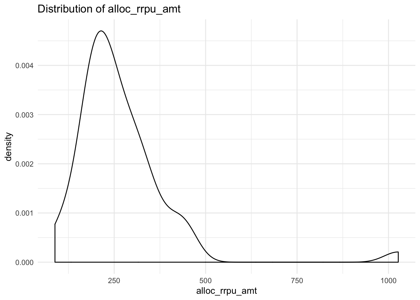

## 
## $alloc_rcm1pu_amt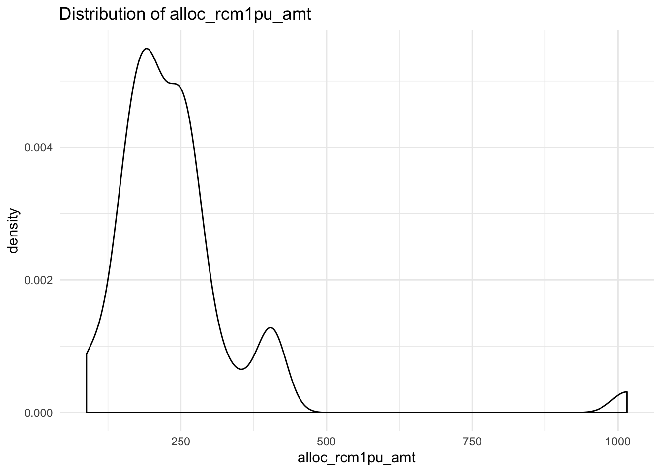

7.17.1 Use function to save plots

We can further manipulate the function to make it save the plots

data_vol_plot <- function(x){
    if(!dir.exists("plots")){
        dir.create("plots")
    }
    
p <-    ggplot(df, aes_string(x = x)) +
        geom_density() +
        theme_minimal() +
        labs(title = paste("Distribution of", x))

ggsave(paste0("plots/", x, ".png"), p)
}

map(cols, data_vol_plot)

## Saving 7 x 5 in image
## Saving 7 x 5 in image

## $alloc_rrpu_amt
## NULL
## 
## $alloc_rcm1pu_amt
## NULL

7.18 Excercise 4

• Using this function:

data_vol_plot <- function(x){
    if(!dir.exists("plots")){
        dir.create("plots")
    }
    p <-    ggplot(df, aes_string(x = x)) +
        geom_density() +
        theme_minimal() +
        labs(title = paste("Distribution of", x))
    
    ggsave(paste0("plots/", x, ".png"), p)
}

• Save all the plots in a folder called plots using the manipulated function

Like this:

map(cols, data_vol_plot)

7.18.1 purrr is powerful

Can be used for:

• Reading in complex excel-workbooks
• Creating many reports for different data-sets
• Applying many models on groups in data

7.19 Scoped verbs

• Sometimes we need want to do things such as calculate the mean of every numeric column
• For this we use dplyr’s scoped verbs.

These are:

• mutate_all()
• mutate_if()
• mutate_at()

These are the same for summarise()/select()/filter()/ arrange()

library(tidyr)
mtcars %>% 
    summarise_all(mean) %>% 
    gather(column, mean)

##    column        mean
## 1     mpg  20.0906250
## 2     cyl   6.1875000
## 3    disp 230.7218750
## 4      hp 146.6875000
## 5    drat   3.5965625
## 6      wt   3.2172500
## 7    qsec  17.8487500
## 8      vs   0.4375000
## 9      am   0.4062500
## 10   gear   3.6875000
## 11   carb   2.8125000
## 12    div   0.9569179

7.19.1 or mutating all columns

mtcars %>% 
    mutate_all(log10)

##         mpg       cyl     disp       hp      drat        wt     qsec   vs
## 1  1.322219 0.7781513 2.204120 2.041393 0.5910646 0.4183013 1.216430 -Inf
## 2  1.322219 0.7781513 2.204120 2.041393 0.5910646 0.4586378 1.230960 -Inf
## 3  1.357935 0.6020600 2.033424 1.968483 0.5854607 0.3654880 1.269746    0
## 4  1.330414 0.7781513 2.411620 2.041393 0.4885507 0.5071810 1.288696    0
## 5  1.271842 0.9030900 2.556303 2.243038 0.4983106 0.5365584 1.230960 -Inf
## 6  1.257679 0.7781513 2.352183 2.021189 0.4409091 0.5390761 1.305781    0
## 7  1.155336 0.9030900 2.556303 2.389166 0.5065050 0.5526682 1.199755 -Inf
## 8  1.387390 0.6020600 2.166430 1.792392 0.5670264 0.5037907 1.301030    0
## 9  1.357935 0.6020600 2.148603 1.977724 0.5932861 0.4983106 1.359835    0
## 10 1.283301 0.7781513 2.224274 2.089905 0.5932861 0.5365584 1.262451    0
## 11 1.250420 0.7781513 2.224274 2.089905 0.5932861 0.5365584 1.276462    0
## 12 1.214844 0.9030900 2.440594 2.255273 0.4871384 0.6095944 1.240549 -Inf
## 13 1.238046 0.9030900 2.440594 2.255273 0.4871384 0.5717088 1.245513 -Inf
## 14 1.181844 0.9030900 2.440594 2.255273 0.4871384 0.5774918 1.255273 -Inf
## 15 1.017033 0.9030900 2.673942 2.311754 0.4668676 0.7201593 1.254790 -Inf
## 16 1.017033 0.9030900 2.662758 2.332438 0.4771213 0.7343197 1.250908 -Inf
## 17 1.167317 0.9030900 2.643453 2.361728 0.5092025 0.7279477 1.241048 -Inf
## 18 1.510545 0.6020600 1.895975 1.819544 0.6106602 0.3424227 1.289366    0
## 19 1.482874 0.6020600 1.879096 1.716003 0.6928469 0.2081725 1.267641    0
## 20 1.530200 0.6020600 1.851870 1.812913 0.6253125 0.2636361 1.298853    0
## 21 1.332438 0.6020600 2.079543 1.986772 0.5682017 0.3918169 1.301247    0
## 22 1.190332 0.9030900 2.502427 2.176091 0.4409091 0.5465427 1.227115 -Inf
## 23 1.181844 0.9030900 2.482874 2.176091 0.4983106 0.5359267 1.238046 -Inf
## 24 1.123852 0.9030900 2.544068 2.389166 0.5717088 0.5843312 1.187803 -Inf
## 25 1.283301 0.9030900 2.602060 2.243038 0.4885507 0.5848963 1.231724 -Inf
## 26 1.436163 0.6020600 1.897627 1.819544 0.6106602 0.2866810 1.276462    0
## 27 1.414973 0.6020600 2.080266 1.959041 0.6464037 0.3304138 1.222716 -Inf
## 28 1.482874 0.6020600 1.978181 2.053078 0.5763414 0.1798389 1.227887    0
## 29 1.198657 0.9030900 2.545307 2.421604 0.6253125 0.5010593 1.161368 -Inf
## 30 1.294466 0.7781513 2.161368 2.243038 0.5587086 0.4424798 1.190332 -Inf
## 31 1.176091 0.9030900 2.478566 2.525045 0.5490033 0.5526682 1.164353 -Inf
## 32 1.330414 0.6020600 2.082785 2.037426 0.6138418 0.4440448 1.269513    0
##      am      gear      carb          div
## 1     0 0.6020600 0.6020600 -0.105789464
## 2     0 0.6020600 0.6020600 -0.091259739
## 3     0 0.6020600 0.0000000 -0.088188474
## 4  -Inf 0.4771213 0.0000000 -0.041717513
## 5  -Inf 0.4771213 0.3010300 -0.040882051
## 6  -Inf 0.4771213 0.0000000  0.048102576
## 7  -Inf 0.4771213 0.6020600  0.044419140
## 8  -Inf 0.6020600 0.3010300 -0.086359831
## 9  -Inf 0.6020600 0.3010300  0.001900635
## 10 -Inf 0.6020600 0.6020600 -0.020850139
## 11 -Inf 0.6020600 0.6020600  0.026041802
## 12 -Inf 0.4771213 0.4771213  0.025705400
## 13 -Inf 0.4771213 0.4771213  0.007466565
## 14 -Inf 0.4771213 0.4771213  0.073428917
## 15 -Inf 0.4771213 0.6020600  0.237756348
## 16 -Inf 0.4771213 0.6020600  0.233874360
## 17 -Inf 0.4771213 0.6020600  0.073730816
## 18    0 0.6020600 0.0000000 -0.221179059
## 19    0 0.6020600 0.3010300 -0.215232601
## 20    0 0.6020600 0.0000000 -0.231346622
## 21 -Inf 0.4771213 0.0000000 -0.031191371
## 22 -Inf 0.4771213 0.3010300  0.036783384
## 23 -Inf 0.4771213 0.3010300  0.056202515
## 24 -Inf 0.4771213 0.6020600  0.063950998
## 25 -Inf 0.4771213 0.3010300 -0.051576845
## 26    0 0.6020600 0.0000000 -0.159700843
## 27    0 0.6989700 0.3010300 -0.192256877
## 28    0 0.6989700 0.3010300 -0.254986879
## 29    0 0.6989700 0.6020600 -0.037289085
## 30    0 0.6989700 0.7781513 -0.104134528
## 31    0 0.6989700 0.9030900 -0.011738403
## 32    0 0.6020600 0.3010300 -0.060900829

mtcars %>% 
    summarise_all(list(~min(.), ~max(.)))

##   mpg_min cyl_min disp_min hp_min drat_min wt_min qsec_min vs_min am_min
## 1    10.4       4     71.1     52     2.76  1.513     14.5      0      0
##   gear_min carb_min   div_min mpg_max cyl_max disp_max hp_max drat_max
## 1        3        1 0.5559211    33.9       8      472    335     4.93
##   wt_max qsec_max vs_max am_max gear_max carb_max  div_max
## 1  5.424     22.9      1      1        5        8 1.728846

mtcars %>% 
    summarise_all(list(~min(.), ~max(.))) %>% 
    gather(colname, value) %>% 
    separate(colname, into = c("colname", "calc"), sep = "_")

##    colname calc       value
## 1      mpg  min  10.4000000
## 2      cyl  min   4.0000000
## 3     disp  min  71.1000000
## 4       hp  min  52.0000000
## 5     drat  min   2.7600000
## 6       wt  min   1.5130000
## 7     qsec  min  14.5000000
## 8       vs  min   0.0000000
## 9       am  min   0.0000000
## 10    gear  min   3.0000000
## 11    carb  min   1.0000000
## 12     div  min   0.5559211
## 13     mpg  max  33.9000000
## 14     cyl  max   8.0000000
## 15    disp  max 472.0000000
## 16      hp  max 335.0000000
## 17    drat  max   4.9300000
## 18      wt  max   5.4240000
## 19    qsec  max  22.9000000
## 20      vs  max   1.0000000
## 21      am  max   1.0000000
## 22    gear  max   5.0000000
## 23    carb  max   8.0000000
## 24     div  max   1.7288462

mtcars %>% 
    summarise_all(~mean(., na.rm = TRUE))

##        mpg    cyl     disp       hp     drat      wt     qsec     vs
## 1 20.09062 6.1875 230.7219 146.6875 3.596563 3.21725 17.84875 0.4375
##        am   gear   carb       div
## 1 0.40625 3.6875 2.8125 0.9569179

7.19.2 Excercise 5

• Calculate the mean on every numeric column in your data frame.

7.20 R and databases

• Databases are great for storing data

• Can do heavy computations on a lot of data

7.20.1 Different strategies

7.20.2 What databases need

• Credentials

• Location

• Driver

For example:

• Credentials - token/userame/network-config

• Location - IP/URL

• Driver - ODBC/JDBC

We will use Spark as a database

library(sparklyr)

## 
## Attaching package: 'sparklyr'

## The following object is masked from 'package:purrr':
## 
##     invoke

sc <- spark_connect(master = "local")

7.21 Copy data to data base

copy_to(sc, nycflights13::flights, "flights")

## # Source: spark<flights> [?? x 19]
##     year month   day dep_time sched_dep_time dep_delay arr_time
##    <int> <int> <int>    <int>          <int>     <dbl>    <int>
##  1  2013     1     1      517            515         2      830
##  2  2013     1     1      533            529         4      850
##  3  2013     1     1      542            540         2      923
##  4  2013     1     1      544            545        -1     1004
##  5  2013     1     1      554            600        -6      812
##  6  2013     1     1      554            558        -4      740
##  7  2013     1     1      555            600        -5      913
##  8  2013     1     1      557            600        -3      709
##  9  2013     1     1      557            600        -3      838
## 10  2013     1     1      558            600        -2      753
## # … with more rows, and 12 more variables: sched_arr_time <int>,
## #   arr_delay <dbl>, carrier <chr>, flight <int>, tailnum <chr>,
## #   origin <chr>, dest <chr>, air_time <dbl>, distance <dbl>, hour <dbl>,
## #   minute <dbl>, time_hour <dttm>

7.22 Once data is in Spark you can use SQL with it

select origin, count(*) as n from flights group by origin

Table 7.1: 3 records

origin	n
JFK	111279
LGA	104662
EWR	120835

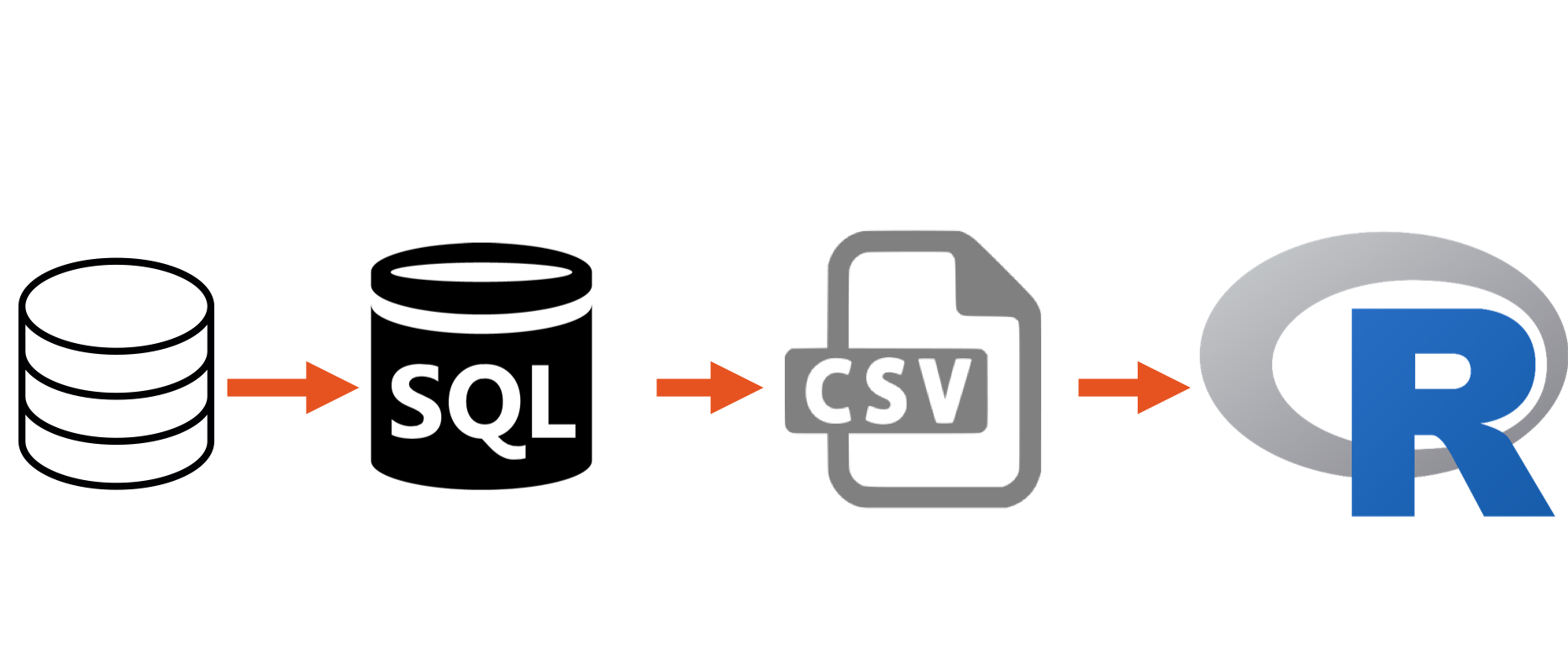
This follows this strategy

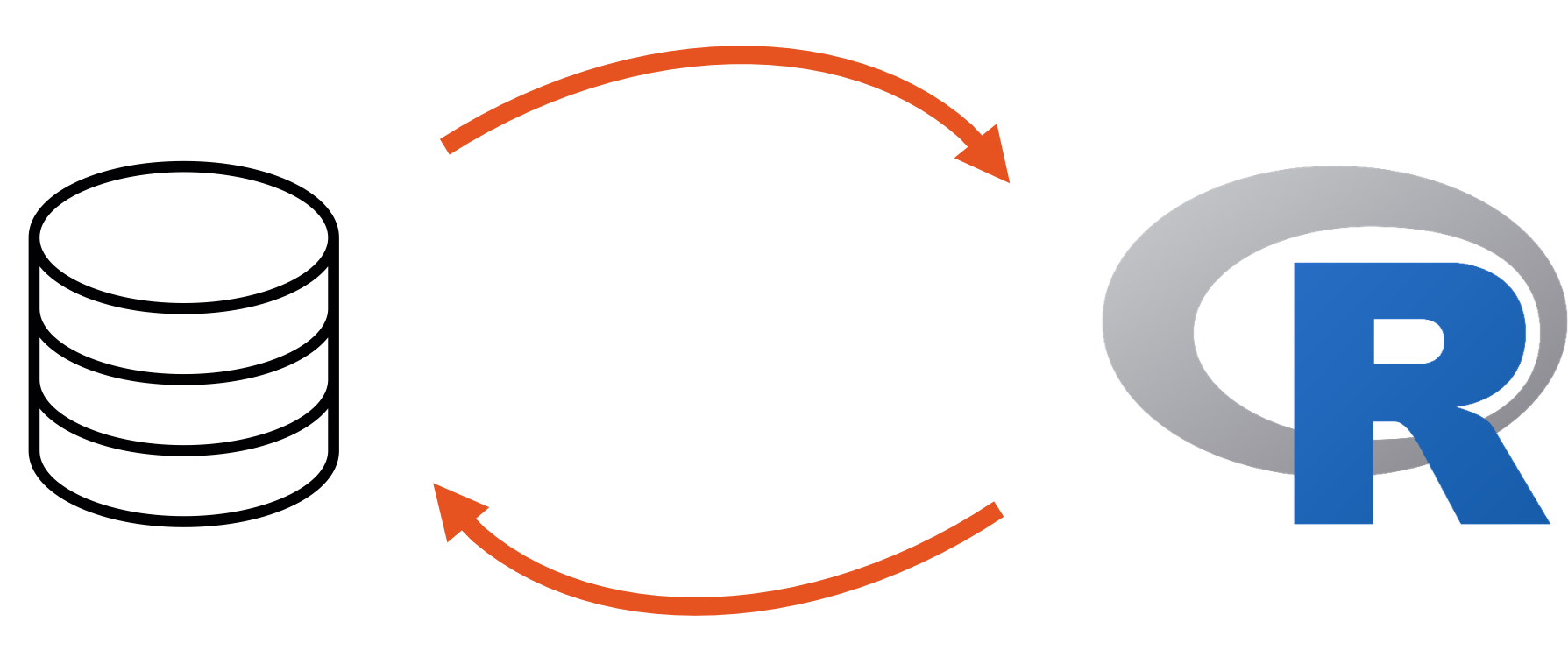
7.22.1 You can use dplyr with SQL as a backend

library(dbplyr)

## 
## Attaching package: 'dbplyr'

## The following objects are masked from 'package:dplyr':
## 
##     ident, sql

flights <- tbl(sc, "flights")

flights %>%
    group_by(origin) %>%
    count()

## # Source: spark<?> [?? x 2]
## # Groups: origin
##   origin      n
##   <chr>   <dbl>
## 1 JFK    111279
## 2 LGA    104662
## 3 EWR    120835

7.22.2 And we can use dplyr’s scoped verbs in Spark

flights %>% 
    select_if(is.numeric) %>% 
    summarise_all(mean) %>% 
    collect() %>% 
    gather(colname, mean)

## Applying predicate on the first 100 rows

## Warning: Missing values are always removed in SQL.
## Use `mean(x, na.rm = TRUE)` to silence this warning
## This warning is displayed only once per session.

## # A tibble: 14 x 2
##    colname           mean
##    <chr>            <dbl>
##  1 year           2013   
##  2 month             6.55
##  3 day              15.7 
##  4 dep_time       1349.  
##  5 sched_dep_time 1344.  
##  6 dep_delay        12.6 
##  7 arr_time       1502.  
##  8 sched_arr_time 1536.  
##  9 arr_delay         6.90
## 10 flight         1972.  
## 11 air_time        151.  
## 12 distance       1040.  
## 13 hour             13.2 
## 14 minute           26.2

7.22.3 We can also read csv-files into Spark using spark_read_csv(sc, name, path)

spark_read_csv(sc, "customers", "data/tele2-kunder.csv")

7.23 Excercise 5

• Connect to your spark-cluster

• read in the data-set tele2-transaction.csv into Spark using spark_read_csv()

• Which is the most common “säljkanal”?

• What’s the mean rrpu for each priceplan?

• How many customers did increase their number of subscriptions when signing a new contract?

• What is the most common bas_bucket_size?

7.24 Manipulating spark data.frames

• A lot of functions in R are translated to SQL when you call them on a database-table

7.24.1 Basic math operators

+, -, *, /, %%, ^

7.24.2 Math functions

abs, acos, asin, asinh, atan, atan2, ceiling, cos, cosh, exp, floor, log, log10, round, sign, sin, sinh, sqrt, tan, tanh

7.24.3 Logical comparisons

<, <=, !=, >=, >, ==, %in%

7.24.4 Boolean operations

&, &&, |, ||, !

7.24.5 Character functions

paste, tolower, toupper, nchar

7.24.6 Casting

as.double, as.integer, as.logical, as.character, as.date

7.24.7 Basic aggregations

mean, sum, min, max, sd, var, cor, cov, n

7.25 This means we can call these functions in mutate() on a Spark data.frame

flights %>% 
    mutate(carrier = tolower(carrier)) %>% 
    select(1:5, carrier)

## # Source: spark<?> [?? x 6]
##     year month   day dep_time sched_dep_time carrier
##    <int> <int> <int>    <int>          <int> <chr>  
##  1  2013     1     1      517            515 ua     
##  2  2013     1     1      533            529 ua     
##  3  2013     1     1      542            540 aa     
##  4  2013     1     1      544            545 b6     
##  5  2013     1     1      554            600 dl     
##  6  2013     1     1      554            558 ua     
##  7  2013     1     1      555            600 b6     
##  8  2013     1     1      557            600 ev     
##  9  2013     1     1      557            600 b6     
## 10  2013     1     1      558            600 aa     
## # … with more rows

flights %>% 
    mutate(date = as.Date(paste(year,"-", month,"-", day))) %>% 
    select(year, month, day, date)

## # Source: spark<?> [?? x 4]
##     year month   day date      
##    <int> <int> <int> <date>    
##  1  2013     1     1 2013-01-01
##  2  2013     1     1 2013-01-01
##  3  2013     1     1 2013-01-01
##  4  2013     1     1 2013-01-01
##  5  2013     1     1 2013-01-01
##  6  2013     1     1 2013-01-01
##  7  2013     1     1 2013-01-01
##  8  2013     1     1 2013-01-01
##  9  2013     1     1 2013-01-01
## 10  2013     1     1 2013-01-01
## # … with more rows

7.26 What dplyr does is just really translating the dplyr-code into SQL

flights %>% 
    mutate(date = as.Date(paste(year,"-", month,"-", day))) %>% 
    select(year, month, day, date) %>% 
    show_query()

## <SQL>
## SELECT `year`, `month`, `day`, CAST(CONCAT_WS(" ", `year`, "-", `month`, "-", `day`) AS DATE) AS `date`
## FROM `flights`

7.27 When do we need to bring data into R?

• Plotting

7.28 How do we collect data into R?

• with collect()

flights %>%
    group_by(origin) %>%
    count() %>% 
    collect() %>% 
    ggplot(aes(x = reorder(origin, -n), y = n)) +
    geom_col() +
    theme_minimal() +
    labs(title = "Number of flights / origin",
                        x = "Origin", 
                        y = "Number of flights")

Or

flights %>%
    mutate(date = as.Date(paste0(as.character(year), "-", as.character(month), "-", as.character(day)))) %>% 
    group_by(date, origin) %>%
    count() %>% 
    collect() %>% 
    ggplot(aes(x = date, y = n, color = origin)) +
    geom_point() + 
    geom_smooth() +
    theme_minimal() +
    labs(title = "Number of flights",
                        x = "Origin", 
                        y = "Number of flights") +
    scale_y_continuous(limits = c(0, 450))

## `geom_smooth()` using method = 'loess' and formula 'y ~ x'

7.29 Visualize distributions in a database

• You can do this with the package dbplot

library(dbplot)

dbplot_histogram(flights, dep_delay)

## Warning: Removed 1 rows containing missing values (position_stack).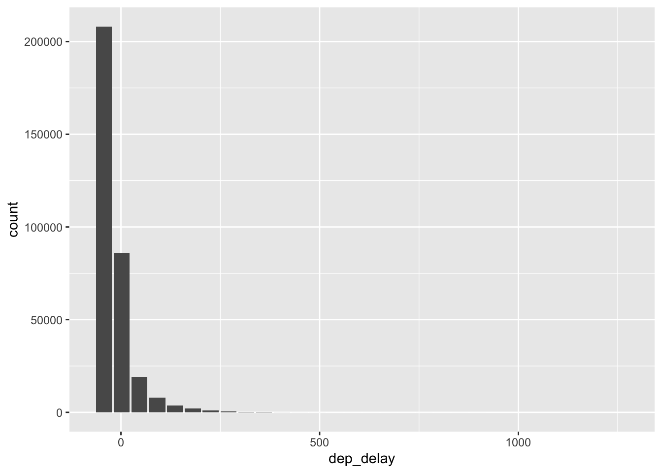

dbplot_raster(flights, dep_delay, arr_delay)

## Warning: Removed 30 rows containing missing values (geom_tile).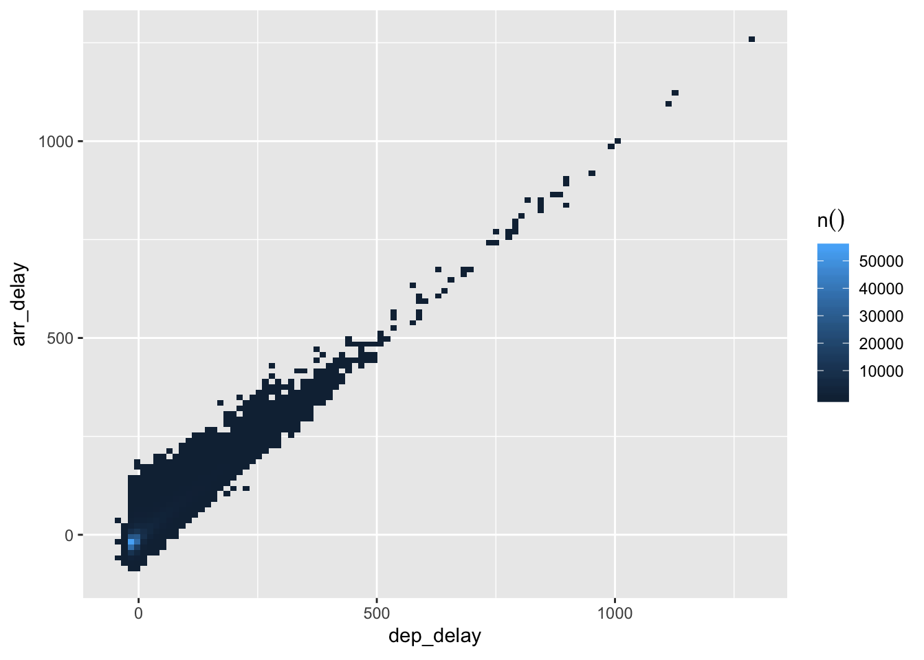

7.30 Excercise 6

• Visualize subscriptions over time, either by day, or month or any other variable you find suitable

• Which priceplan is most profitable? Visualize

• What is the most common customer type? Visualize

• Can you visualize any numerical relationships in the data?

7.31 Extra

• Explore the transactions data-set
• Make 4 visualizations that tells a story about this data-set
• If you have time, try out the package flexdashboard and turn your four visualizations into a dashboard with sparklyr as a backend.
• I have set up a dashboard-file for you to continue with, you can download it here: https://github.com/Ferrologic/flexdashboard-tele2

7.32 Facit advanced data manipulations

7.32.1 Excercise 1

• Create a functions called my_mean() that has mean(x, na.rm = TRUE) as default
• Create a vector with NA and use it on it

my_function <- function(x){
    log10(x)
}

my_mean <- function(x){
    mean(x, na.rm = T)
}

x <- c(rnorm(100), rep(NA, 10))

my_mean(x)

## [1] -0.1408428

7.32.2 Excercise 2

• Create a function that scales a vector
• Use your function on the data-set tele2-kunder.csv

(df$tr_tot_data_vol_all_netw_2 -
        min(df$tr_tot_data_vol_all_netw_2, na.rm = TRUE)) / 
    (max(df$tr_tot_data_vol_all_netw_2, na.rm = TRUE) -
            min(df$tr_tot_data_vol_all_netw_2, na.rm = TRUE))

scale_vector <- function(x){
    (x -
        min(x, na.rm = TRUE)) / 
    (max(x, na.rm = TRUE) -
            min(x, na.rm = TRUE))
}

scale_vector(x)

##   [1] 0.48759965 0.07138241 0.31716348 0.46929592 0.32039189 0.15150801
##   [7] 0.33335465 0.24057149 0.53296593 0.29368642 0.15274015 1.00000000
##  [13] 0.28566758 0.61719235 0.28498834 0.49749998 0.54362853 0.43417857
##  [19] 0.45108149 0.29380767 0.18845253 0.34592773 0.56154395 0.37484007
##  [25] 0.11758121 0.44794172 0.81734750 0.32088468 0.18346424 0.28962714
##  [31] 0.41973885 0.73729308 0.47884044 0.22707054 0.07897952 0.29641309
##  [37] 0.22190696 0.72066895 0.00000000 0.43248430 0.32070481 0.02051455
##  [43] 0.64354132 0.52026814 0.23037616 0.40923294 0.16434551 0.62762436
##  [49] 0.01036543 0.43683015 0.20593791 0.09344743 0.30527104 0.05249077
##  [55] 0.54582185 0.23478171 0.43035853 0.60224484 0.20462079 0.30158595
##  [61] 0.45609084 0.02845019 0.23845682 0.36423597 0.62984197 0.40832348
##  [67] 0.60718890 0.47947916 0.32906815 0.14540373 0.26220457 0.52006005
##  [73] 0.43676457 0.17114527 0.47926092 0.35597789 0.62987377 0.63207230
##  [79] 0.27355137 0.30428798 0.50476594 0.23095888 0.06911469 0.79081748
##  [85] 0.81988563 0.29283427 0.16048760 0.44379826 0.17289093 0.52759973
##  [91] 0.16751942 0.39802162 0.15513719 0.73383755 0.56431791 0.27799104
##  [97] 0.13832932 0.54948085 0.19746301 0.21128377         NA         NA
## [103]         NA         NA         NA         NA         NA         NA
## [109]         NA         NA

7.32.3 Excercise 3

• Write a function called praise that has a logical input: happy that can be either TRUE or FALSE
• If TRUE return an encouraging text with print("some text")
• If FALSE an even more encouraging text with print("some text")
• Remember: to check if something is TRUE use isTRUE() not x == TRUE

praise(happy = FALSE)

## [1] "Get yourself together you lazy schmuck!"

7.32.4 Excercise 4

• Manipulate the function below so that it generates a bar chart visualizing the summary statitics

Make sure the plot

• Flips the coord for visability
• Displays the groups in order

library(dplyr)
library(ggplot2)
groupwise_rrpu_summary <- function(df, group){
        group_by({{df}}, {{group}}) %>% #<<
        summarise(mean_rrpu = mean(alloc_rrpu_amt, na.rm = T)) %>% 
        ggplot(aes(x = reorder({{group}}, mean_rrpu), y = mean_rrpu)) +
        geom_col() +
        theme_minimal() 
}

groupwise_rrpu_summary(df, cpe_type) +
        coord_flip()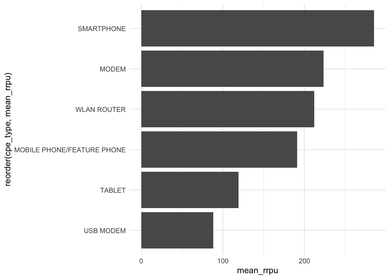

7.32.5 Excercise 3

We want to iterate this function over all the data_vol-columns

• Create a named vector with all the data_vol-columns, use colnames()

cols <- df %>% 
    select(contains("tr_tot_data")) %>% 
    colnames() %>% 
    set_names()

• Apply the plot-function on every column

data_vol_plot <- function(x){
    
    ggplot(df, aes_string(x = x)) +
        geom_density() +
        theme_minimal() +
        labs(title = paste("Distribution of", x))
}

map(cols, data_vol_plot)

## $tr_tot_data_vol_all_netw_1

## Warning: Removed 3 rows containing non-finite values (stat_density).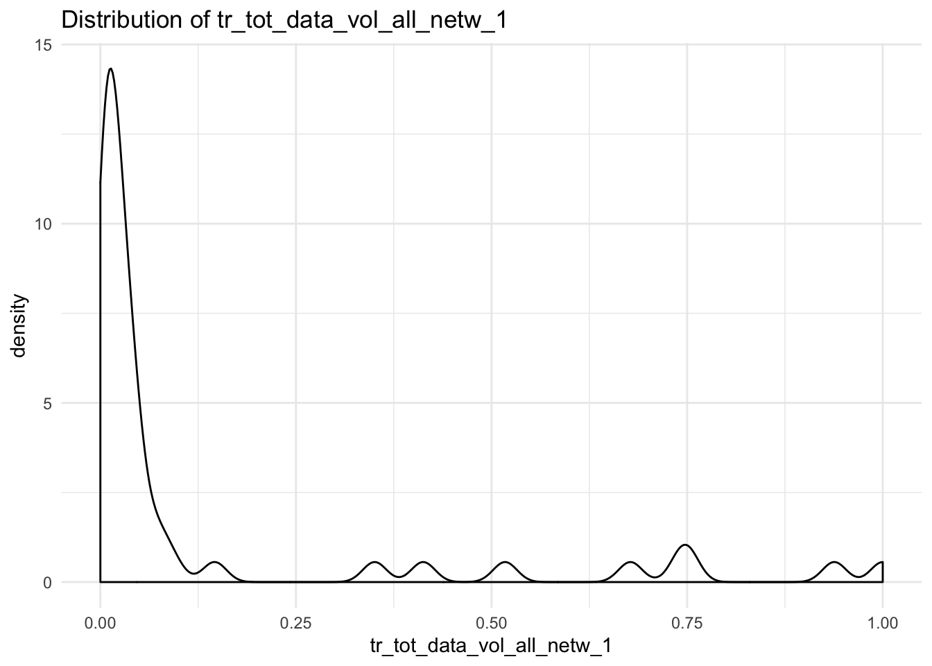

## 
## $tr_tot_data_vol_all_netw_2

## Warning: Removed 3 rows containing non-finite values (stat_density).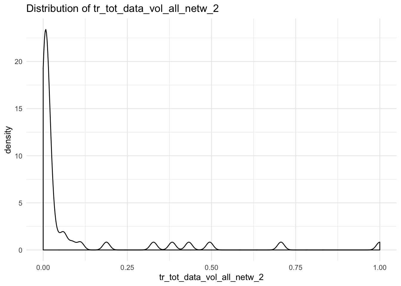

## 
## $tr_tot_data_vol_all_netw_3

## Warning: Removed 1 rows containing non-finite values (stat_density).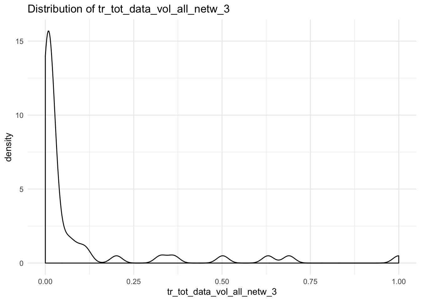

## 
## $tr_tot_data_vol_all_netw_4

## Warning: Removed 3 rows containing non-finite values (stat_density).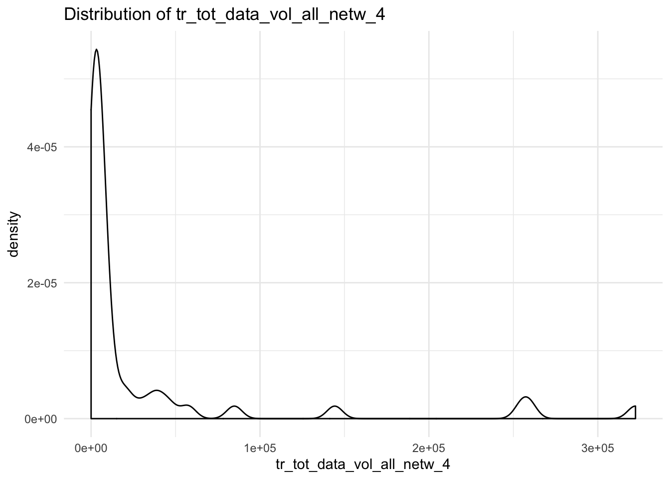

## 
## $tr_tot_data_vol_all_netw_5

## Warning: Removed 4 rows containing non-finite values (stat_density).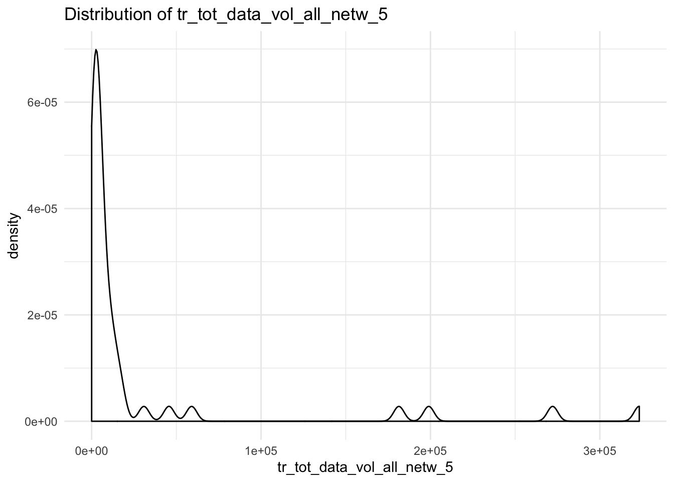

## 
## $tr_tot_data_vol_all_netw_6

## Warning: Removed 4 rows containing non-finite values (stat_density).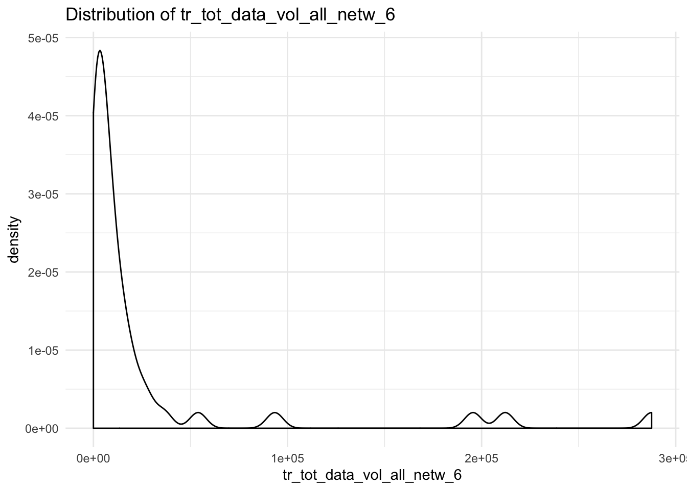

## 
## $tr_tot_data_vol_all_netw_7

## Warning: Removed 4 rows containing non-finite values (stat_density).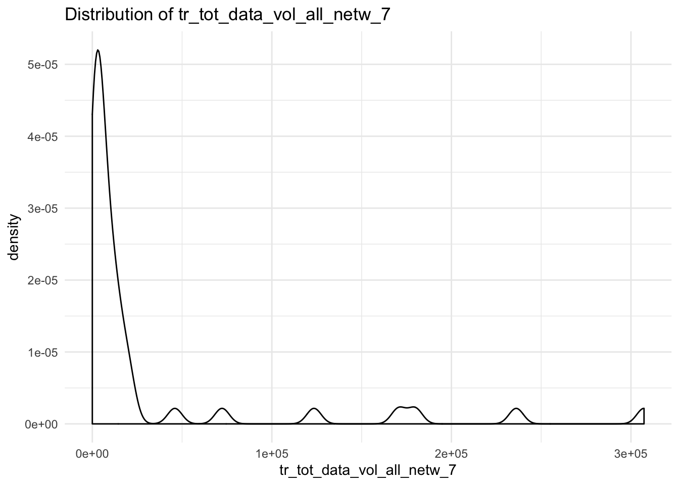

## 
## $tr_tot_data_vol_all_netw_8

## Warning: Removed 4 rows containing non-finite values (stat_density).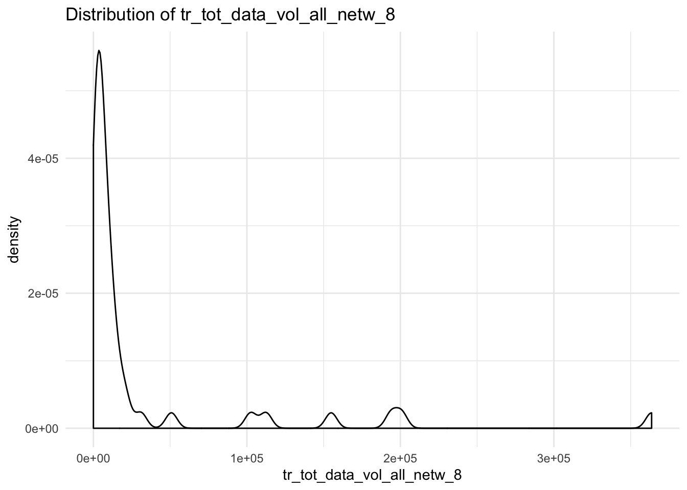

## 
## $tr_tot_data_vol_all_netw_9

## Warning: Removed 4 rows containing non-finite values (stat_density).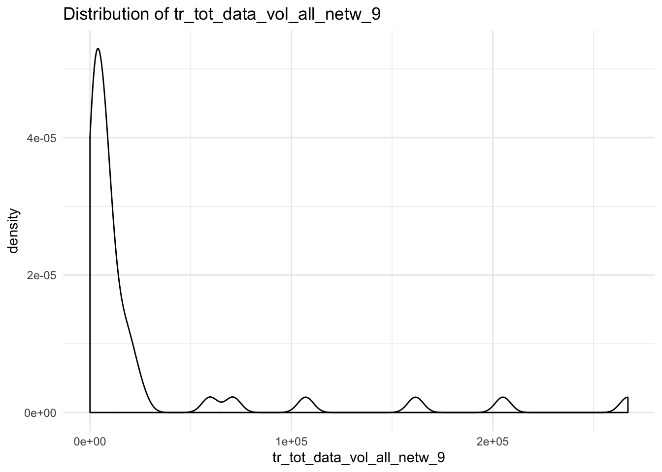

## 
## $tr_tot_data_vol_all_netw_10

## Warning: Removed 4 rows containing non-finite values (stat_density).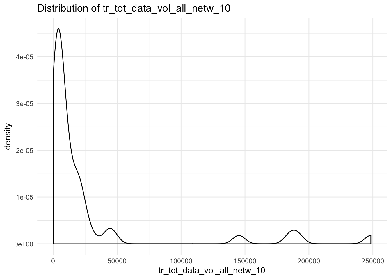

## 
## $tr_tot_data_vol_all_netw_11

## Warning: Removed 4 rows containing non-finite values (stat_density).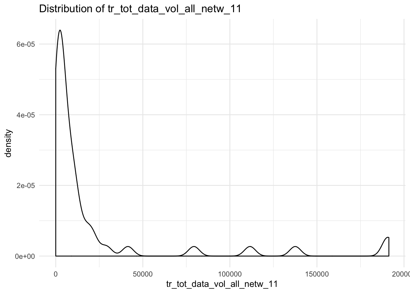

## 
## $tr_tot_data_vol_all_netw_12

## Warning: Removed 5 rows containing non-finite values (stat_density).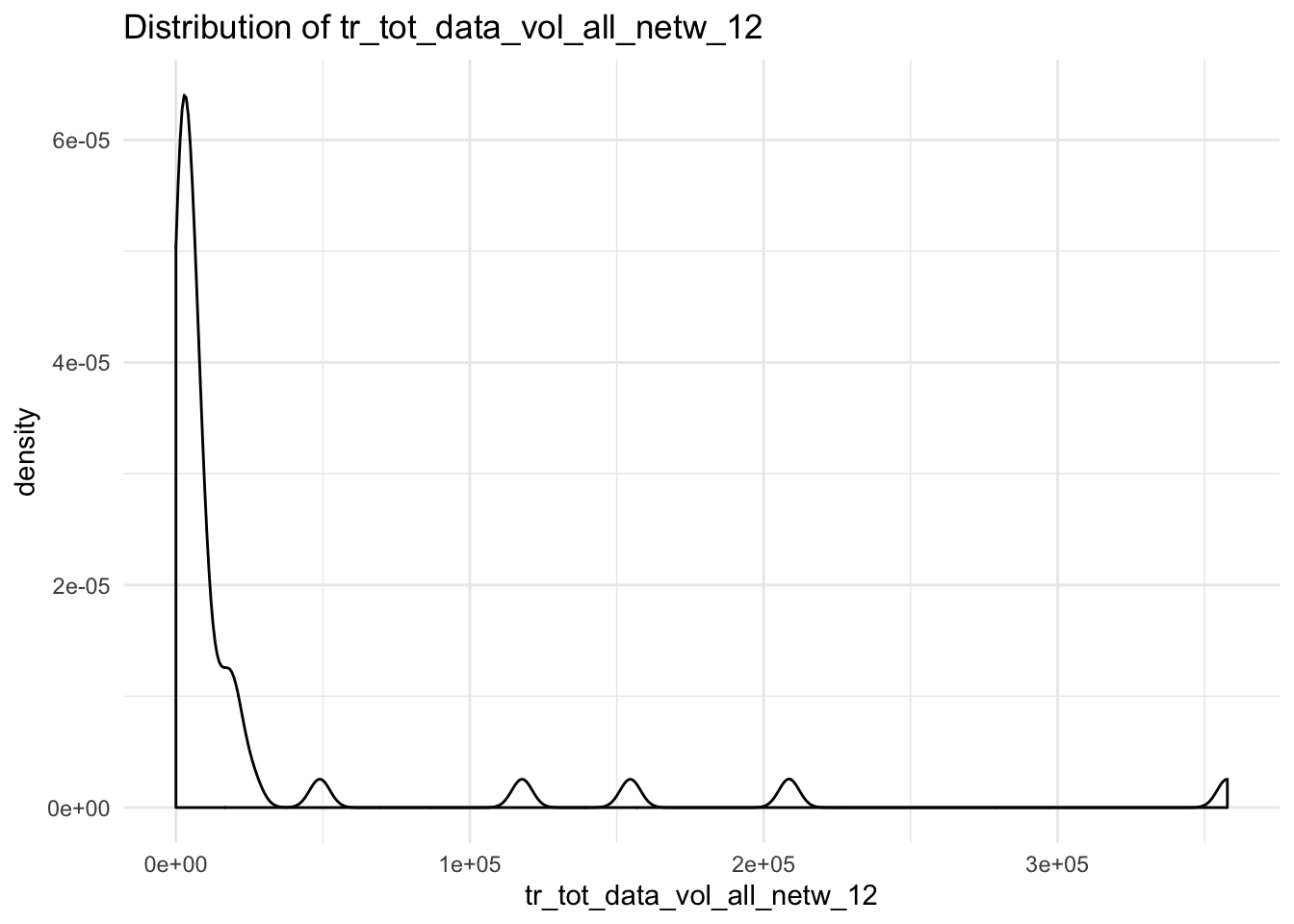

7.32.6 Excercise 4

• Using this function:

data_vol_plot <- function(x){
    if(!dir.exists("plots")){
        dir.create("plots")
    }
    p <-    ggplot(df, aes_string(x = x)) +
        geom_density() +
        theme_minimal() +
        labs(title = paste("Distribution of", x))
    
    ggsave(paste0("plots/", x, ".png"), p)
}

• Save all the plots in a folder called plots using the manipulated function

map(cols, data_vol_plot)

7.32.7 Excercise 5

• Calculate the mean and standard deviation on every numeric column in your data frame.

df %>% 
    summarise_if(is.numeric, list(~mean(., na.rm = T), ~sd(., na.rm = T))) %>% 
    gather(column, value)

## # A tibble: 28 x 2
##    column                                value
##    <chr>                                 <dbl>
##  1 tr_tot_data_vol_all_netw_1_mean      0.136 
##  2 tr_tot_data_vol_all_netw_2_mean      0.0897
##  3 tr_tot_data_vol_all_netw_3_mean      0.0936
##  4 tr_tot_data_vol_all_netw_4_mean  30779.    
##  5 tr_tot_data_vol_all_netw_5_mean  28329.    
##  6 tr_tot_data_vol_all_netw_6_mean  25449.    
##  7 tr_tot_data_vol_all_netw_7_mean  30058.    
##  8 tr_tot_data_vol_all_netw_8_mean  31373.    
##  9 tr_tot_data_vol_all_netw_9_mean  25142.    
## 10 tr_tot_data_vol_all_netw_10_mean 25794.    
## # … with 18 more rows

7.32.8 Excercise 6

• Create a local spark connection
• read the data-set tele2-transaction.csv into Spark using spark_read_csv()

library(sparklyr)
sc <- spark_connect(master = "local")

## Re-using existing Spark connection to local

spark_read_csv(sc, "transactions", "data/tele2-transactions.csv")

## # Source: spark<transactions> [?? x 11]
##    su_contract_dt      ar_key cust_id false_gi increasednosub
##    <dttm>              <chr>  <chr>      <int>          <int>
##  1 2017-10-31 23:00:00 AAEBf… AAEBft…        0              1
##  2 2019-02-16 23:00:00 AAEBf… AAEBfp…        0              1
##  3 2017-07-17 22:00:00 AAEBf… AAEBfp…        0              1
##  4 2018-02-12 23:00:00 AAEBf… AAEBfn…        0              1
##  5 2018-05-01 22:00:00 AAEBf… AAEBfm…        0              1
##  6 2018-11-26 23:00:00 AAEBf… AAEBft…        0              1
##  7 2018-07-30 22:00:00 AAEBf… AAEBfk…        0              1
##  8 2017-11-05 23:00:00 AAEBf… AAEBfq…        0              1
##  9 2017-12-19 23:00:00 AAEBf… AAEBfo…        0              0
## 10 2019-03-13 23:00:00 AAEBf… AAEBft…        0              1
## # … with more rows, and 6 more variables: pc_l3_pd_spec_nm <chr>,
## #   cust_tp <chr>, sc_l5_sales_cnl <chr>, pc_priceplan_nm <chr>,
## #   bas_buck_size <chr>, rrpu <dbl>

trans <- tbl(sc, "transactions")

• Which is the most common “säljkanal”?

trans %>% 
    group_by(sc_l5_sales_cnl) %>% 
    count(sort = TRUE)

## # Source:     spark<?> [?? x 2]
## # Groups:     sc_l5_sales_cnl
## # Ordered by: desc(n)
##    sc_l5_sales_cnl      n
##    <chr>            <dbl>
##  1 CUST_CARE       170089
##  2 PARTNER_SALES    44612
##  3 CO_SALES         24190
##  4 OWN_STORES       18442
##  5 DIRECT_SALES      7185
##  6 RETAILER          6325
##  7 TELEMARKET        4388
##  8 INTERNET_STORE    3289
##  9 MISC               715
## 10 TELESALES1         601
## # … with more rows

• What’s the mean rrpu for each priceplan?

trans %>% 
    group_by(pc_priceplan_nm) %>% 
    summarise(mean_rrpu = mean(rrpu, na.rm = T)) %>% 
    arrange(-mean_rrpu)

## # Source:     spark<?> [?? x 2]
## # Ordered by: -mean_rrpu
##    pc_priceplan_nm                mean_rrpu
##    <chr>                              <dbl>
##  1 Tele2 Myndighet f Tillg Medier     2285.
##  2 Tele2 Husqvarna AB Large           1280.
##  3 Låg Utland                         1102.
##  4 Mobil XL                            627.
##  5 Fast pris Norden 100 GB             604.
##  6 MBB 500 GB                          584.
##  7 Affärspaket Large                   581.
##  8 Fast Pris Norden 100GB              581.
##  9 Fast Pris Norden 50GB               551.
## 10 Fast pris Norden 50 GB              551.
## # … with more rows

• How many customers did increase their number of subscriptions when signing a new contract?

trans %>% 
    group_by(increasednosub) %>% 
    count()

## # Source: spark<?> [?? x 2]
## # Groups: increasednosub
##   increasednosub      n
##            <int>  <dbl>
## 1              1 230084
## 2              0  51557

• What is the most common bas_bucket_size?

trans %>% 
    group_by(bas_buck_size) %>% 
    count(sort = TRUE)

## # Source:     spark<?> [?? x 2]
## # Groups:     bas_buck_size
## # Ordered by: desc(n)
##    bas_buck_size     n
##    <chr>         <dbl>
##  1 1             48950
##  2 7             45117
##  3 5             26096
##  4 0             26023
##  5 10            23922
##  6 50            13938
##  7 Unlimited     13181
##  8 30            12490
##  9 3             12451
## 10 15            11582
## # … with more rows

´ ### Excercise 6

• Visualize subscriptions over time, either by day, or month or any other variable you find suitable

trans %>% 
    mutate(date = as.Date(su_contract_dt)) %>% 
    group_by(date) %>% 
    summarise(count = n()) %>% 
    collect() %>% 
    ungroup() %>% 
    mutate(month = lubridate::floor_date(date, "months")) %>% 
    group_by(month) %>% 
    summarise(count = sum(count)) %>% 
    ggplot(aes(x = month, y = count)) +
    geom_line()

## Warning: Removed 1 rows containing missing values (geom_path).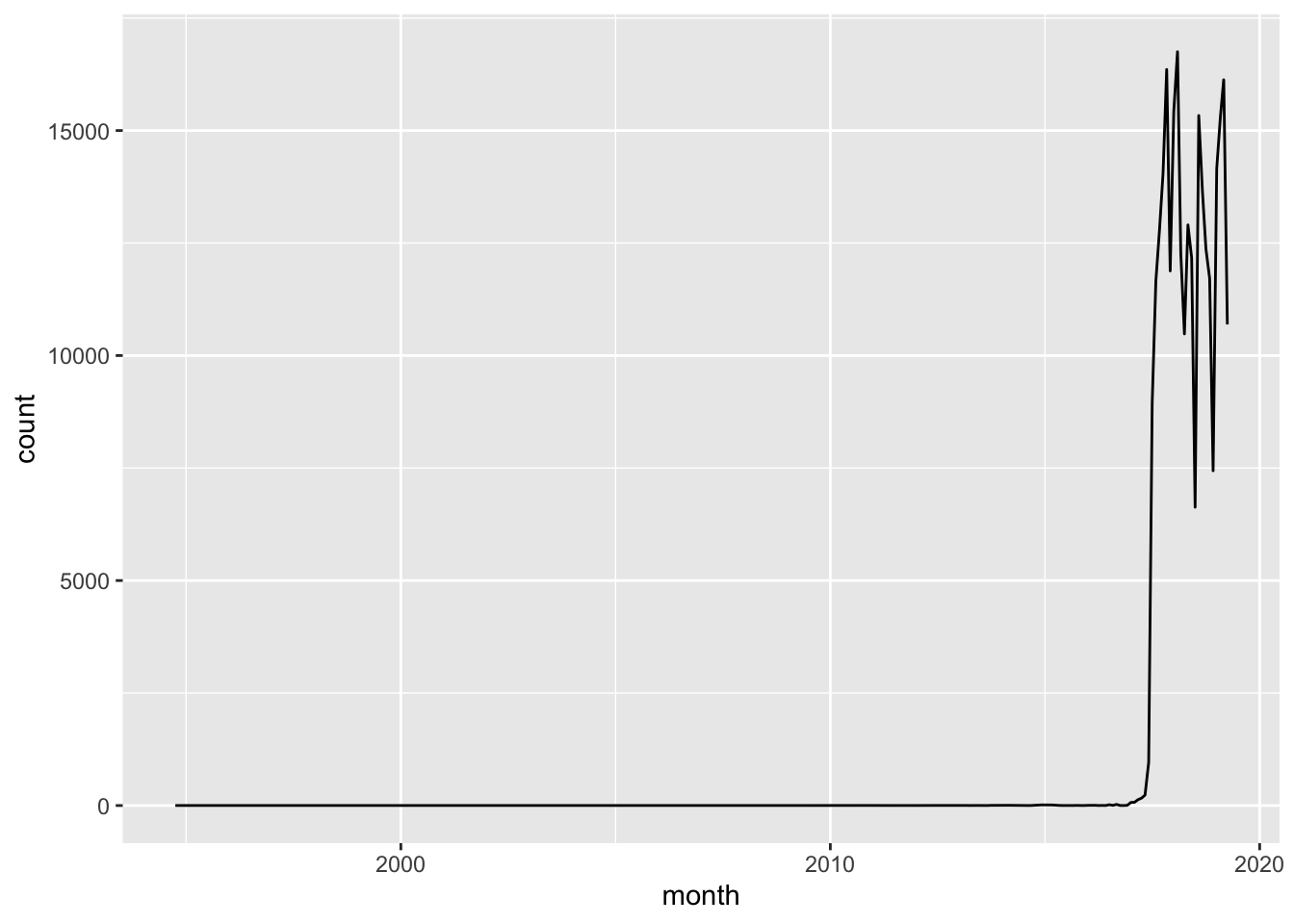

• Which top 10 priceplans are most profitable? Visualize (you can use dplyr function top_n() to get the top 10 of a data.frame)

trans %>% 
    group_by(pc_priceplan_nm) %>% 
    summarise(mean_rrpu = mean(rrpu, na.rm = T)) %>% 
    collect() %>% 
    top_n(10) %>% 
    ggplot(aes(reorder(pc_priceplan_nm, mean_rrpu), y = mean_rrpu)) +
    geom_col() +
    coord_flip()

## Selecting by mean_rrpu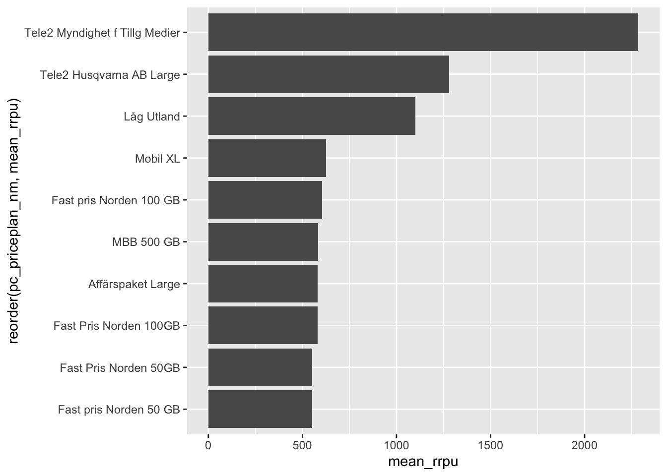

• What is the most common customer type? Visualize

trans %>% 
    group_by(cust_tp) %>% 
    count() %>% 
    collect() %>% 
    ggplot(aes(x = reorder(cust_tp, n), y = n)) +
    geom_col()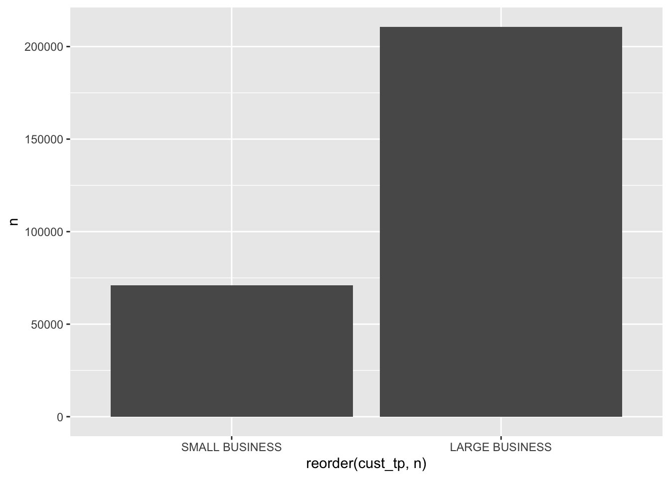

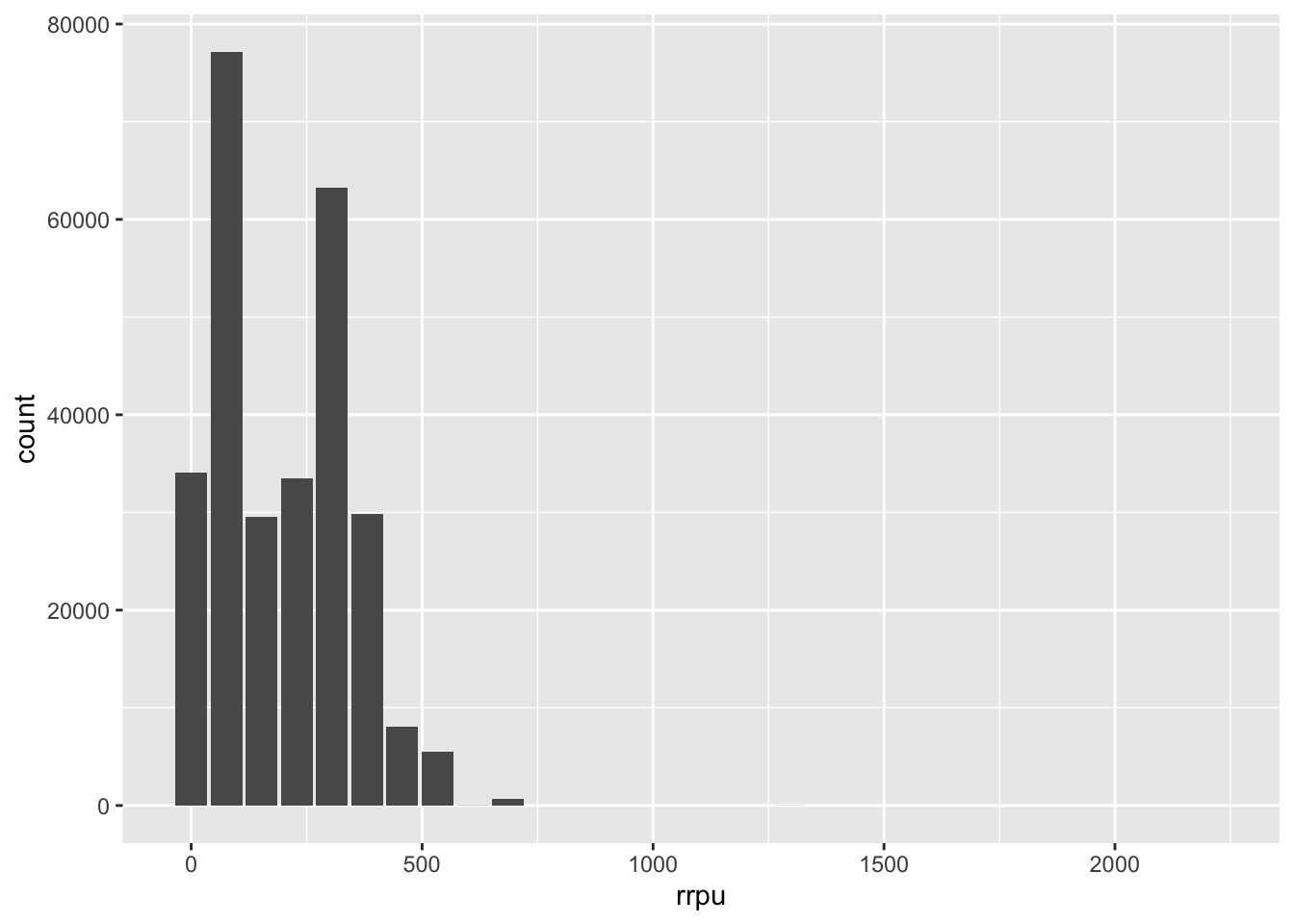
• Visualie the distribution of rrpu, use dbplot

library(dbplot)

dbplot_histogram(trans, rrpu)