2 Introduction to R
In this introductory chapter, you will learn:
- how to import data
- how to manipulate a dataset with the pipe operator
- how to summarize a dataset
- how to make scatterplots and histograms
2.1 Importing data
In this chapter, we will explore a publicly available dataset of Airbnb data. We found these data here. (These are real data “scraped” from airbnb.com in July 2017. This means that the website owner created a script to automatically collect these data from the airbnb.com website. This is one of the many things that you can also do in R. But first let’s learn the basics.) You can download the dataset by right-clicking on this link, selecting “Save link as…” (or something similar), and saving the .csv file in a directory on your hard drive. As mentioned in the introduction, it’s a good idea to save your work in a directory that is automatically backed up by file-sharing software. Later on, we will save our script in the same directory.
2.1.1 Importing CSV files
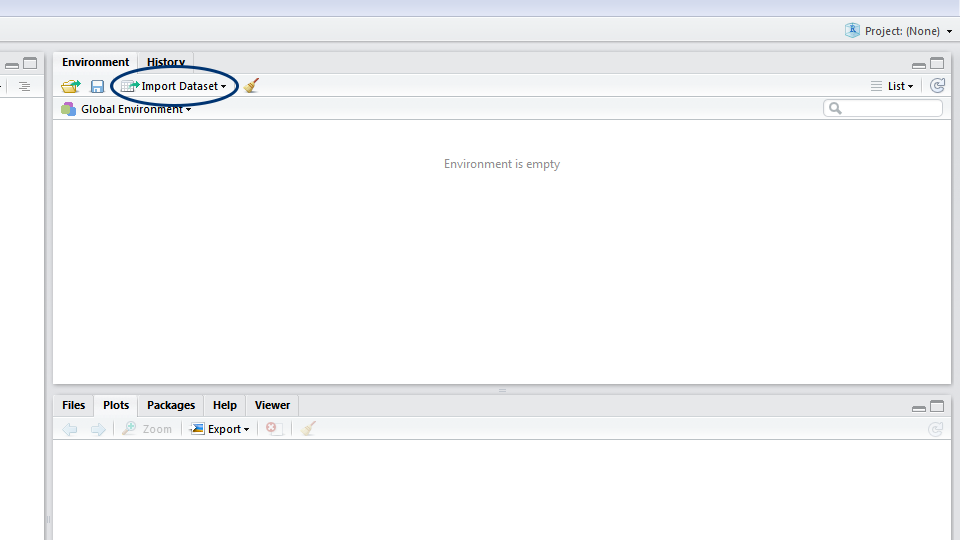
To import data into R, click on Import dataset and then on From text (readr). A new window will pop up. Click on Browse and find your data file. Make sure that First row as names is selected (this tells R to treat the first row of your data as the titles of the columns) and then click on Import. After clicking on import, RStudio opens a Viewer tab. This shows you your data in a spreadsheet.
Some computers save .csv files with semicolons (;) instead of commas (,) as the separators or ‘delimiters’. This usually happens when English is not the first or only language on your computer. If your files are separated by semicolons, click on Import Dataset and find your data file, but now choose Semicolon in the dropdown menu Delimiter.
Note: if you did not save the dataset by right-clicking the link and selecting “Save link as…”, but instead left-clicked the link, then your browser may have ended up opening the dataset. You could then save the dataset by pressing Ctrl+S. Note, however, that your browser may end up saving the dataset as a .txt file. It’s important to then change the extension of your file in the arguments to the read_csv command below.
2.1.2 Setting your working directory
After you have imported your data with Import dataset, check the console window. You’ll see the command for opening the Viewer (View()), and one line above that, you’ll see the command that reads the data. Copy the command that reads the data from the console to your script. In my case it looks like this:
tomslee_airbnb_belgium_1454_2017_07_14 <- read_csv("c:/Dropbox/work/teaching/R/data/tomslee_airbnb_belgium_1454_2017-07-14.csv")
# Change .csv to .txt if necessary.
This line reads as follows (from right to left): the read_csv function should read the tomslee_airbnb_belgium_1454_2017-07-14.csv file from the c:/Dropbox/work/teaching/R/data/ directory (you will see a different directory here). Then, R should assign (<-) these data to an object named tomslee_airbnb_belgium_1454_2017_07_14.
Before we explain each of these concepts, let’s simplify this line of code:
setwd("c:/Dropbox/work/teaching/R/data/") # Set the working directory to where R needs to look for the .csv file
airbnb <- read_csv("tomslee_airbnb_belgium_1454_2017-07-14.csv")
# read_csv now does not require a directory anymore and only needs a filename.
# We assign the data to an object with a simpler name: airbnb instead of tomslee_airbnb_belgium_1454_2017_07_14
The setwd command tells R where your working directory is. Your working directory is a folder on your computer where R will look for data, where plots will be saved, etc. Set your working directory to the folder where you have stored your data. Now, the read_csv file does not require a directory anymore.
You only need to set your working directory once, at the top of your script. You can check whether it’s correctly set by running getwd(). Note that on a Windows computer, file paths have backslashes separating the folders ("C:\folder\data"). However, the filepath you enter into R should use forward slashes ("C:/folder/data").
Save this script in the working directory (in my case: c:/Dropbox/work/teaching/R/data/). In the future you can just run these lines of code to import your data instead of clicking on Import dataset (running lines of code is much faster than pointing and clicking — one of the advantages of using R).
Don’t forget to load the tidyverse package at the top of your script (even before setting the working directory) with library(tidyverse).
2.1.3 Assigning data to objects
Note the <- arrow in the middle of the line that imported the .csv file:
airbnb <- read_csv("tomslee_airbnb_belgium_1454_2017-07-14.csv")<- is the assignment operator. In this case we assign the dataset (i.e., the data we read from the .csv file) to an object named airbnb. An object is a data structure. All the objects you create will show up in the Environment pane (the top right window). RStudio provides a shortcut for writing <-: Alt + - (in Windows). It’s a good idea to learn this shortcut by heart.
When you import data into R, it will become an object called a data frame. A data frame is like a table or an Excel sheet. It has two dimensions: rows and columns. Usually, the rows represent your observations, the columns represent the different variables. When your data consists of only one dimension (e.g., a sequence of numbers or words), it gets stored in a second type of object called a vector. Later on, we’ll learn how to create vectors.
2.1.4 Importing Excel files
R works best with .csv (comma separated values) files. However, data is often stored as an Excel file (you can download the Airbnb dataset as an Excel file here). R can handle that as well, but you’ll need to load a package called readxl first (this package is part of the tidyverse package, but it does not load with library(tidyverse) because it is not a core tidyverse package):
library(readxl) # load the package

airbnb.excel <- read_excel(path = "tomslee_airbnb_belgium_1454_2017-07-14.xlsx", sheet = "Sheet1")
# make sure the Excel file is saved in your working directory

# you can also leave out path = & sheet =
# then the command becomes: read_excel("tomslee_airbnb_belgium_1454_2017-07-14.xlsx", "Sheet1")
read_excel is a function from the readxl package. It takes two arguments: the first one is the filename and the second argument is the name of the Excel sheet that you want to read.
2.1.5 Inspecting the Airbnb dataset
Our dataset contains information on rooms in Belgium listed on airbnb.com. We know for each room (identified by room_id): who the host is (host_id), what type of room it is (room_type), where it is located (country, city, neighborhood, and even the exact latitude and longitude), how many reviews it has received (reviews), how satisfied people were (overall_satisfaction), price (price), and room characteristics (accommodates, bedrooms, bathrooms, minstay).
A really important step is to check that your data were imported correctly. It’s good practice to always inspect your data — do you see any missing values, do the numbers and names make sense? If you start right away with the analysis, you run the risk of having to re-do your analysis because the data weren’t read correctly, or worse, analysing wrong data without noticing.
airbnb # Print the content of the object airbnb.## # A tibble: 17,651 × 20
## room_id survey_id host_id room_…¹ country city borough neigh…² reviews overa…³ accom…⁴ bedro…⁵ bathr…⁶
## <dbl> <dbl> <dbl> <chr> <lgl> <chr> <chr> <chr> <dbl> <dbl> <dbl> <dbl> <lgl>
## 1 5141135 1454 20676997 Shared… NA Belg… Gent Gent 9 4.5 2 1 NA
## 2 13128333 1454 46098805 Shared… NA Belg… Brussel Schaar… 2 0 2 1 NA
## 3 8298885 1454 30924336 Shared… NA Belg… Brussel Elsene 12 4 2 1 NA
## 4 13822088 1454 81440431 Shared… NA Belg… Oosten… Middel… 19 4.5 4 1 NA
## 5 18324301 1454 14294054 Shared… NA Belg… Brussel Anderl… 5 5 2 1 NA
## 6 12664969 1454 68810179 Shared… NA Belg… Brussel Koekel… 28 5 4 1 NA
## 7 15452889 1454 99127166 Shared… NA Belg… Gent Gent 2 0 2 1 NA
## 8 3911778 1454 3690027 Shared… NA Belg… Brussel Elsene 13 4 2 1 NA
## 9 14929414 1454 30624501 Shared… NA Belg… Vervie… Baelen 2 0 8 1 NA
## 10 8497852 1454 40513093 Shared… NA Belg… Brussel Etterb… 57 4.5 3 1 NA
## # … with 17,641 more rows, 7 more variables: price <dbl>, minstay <lgl>, name <chr>, last_modified <chr>,
## # latitude <dbl>, longitude <dbl>, location <chr>, and abbreviated variable names ¹room_type,
## # ²neighborhood, ³overall_satisfaction, ⁴accommodates, ⁵bedrooms, ⁶bathroomsR tells us we are dealing with a tibble (this is just another word for data frame) with 17651 rows or observations and 20 columns or variables. For each column, the type of the variable is given: int (integer), chr (character), dbl (double), dttm (date-time). Integer and double variables store numbers (integer for round numbers, double for numbers with decimals), character variables store letters, date-time variables store dates and/or times.
R only prints the data of the first ten rows and the maximum number of columns that fit on the screen. If, however, you want to inspect the whole dataset, double-click on the airbnb object in the Environment pane (the top right window) to open open a Viewer tab or run View(airbnb). Mind the capital V in the View command. R is always case-sensitive!
You can also use the print command to ask for more (or less) rows and columns in the console window:
# Print 25 rows (set to Inf to print all rows) & set width to 100 to see more columns.
# Notice that columns that don't fit on the first screen with 25 rows
# are printed below the initial 25 rows.

print(airbnb, n = 25, width = 100)
## # A tibble: 17,651 × 20
## room_id survey_id host_id room_…¹ country city borough neigh…² reviews overa…³ accom…⁴ bedro…⁵
## <dbl> <dbl> <dbl> <chr> <lgl> <chr> <chr> <chr> <dbl> <dbl> <dbl> <dbl>
## 1 5141135 1454 2.07e7 Shared… NA Belg… Gent Gent 9 4.5 2 1
## 2 13128333 1454 4.61e7 Shared… NA Belg… Brussel Schaar… 2 0 2 1
## 3 8298885 1454 3.09e7 Shared… NA Belg… Brussel Elsene 12 4 2 1
## 4 13822088 1454 8.14e7 Shared… NA Belg… Oosten… Middel… 19 4.5 4 1
## 5 18324301 1454 1.43e7 Shared… NA Belg… Brussel Anderl… 5 5 2 1
## 6 12664969 1454 6.88e7 Shared… NA Belg… Brussel Koekel… 28 5 4 1
## 7 15452889 1454 9.91e7 Shared… NA Belg… Gent Gent 2 0 2 1
## 8 3911778 1454 3.69e6 Shared… NA Belg… Brussel Elsene 13 4 2 1
## 9 14929414 1454 3.06e7 Shared… NA Belg… Vervie… Baelen 2 0 8 1
## 10 8497852 1454 4.05e7 Shared… NA Belg… Brussel Etterb… 57 4.5 3 1
## 11 19372053 1454 1.87e7 Shared… NA Belg… Tournai Bruneh… 1 0 4 1
## 12 19855549 1454 1.29e8 Shared… NA Belg… Brussel Etterb… 0 0 2 1
## 13 6772358 1454 3.50e7 Shared… NA Belg… Gent Gent 143 5 2 1
## 14 13852832 1454 8.18e7 Shared… NA Belg… Arlon Arlon 0 0 1 1
## 15 11581251 1454 5.00e7 Shared… NA Belg… Kortri… Waregem 1 0 4 1
## 16 3645177 1454 1.84e7 Shared… NA Belg… Antwer… Boom 3 4.5 2 1
## 17 12032748 1454 6.37e7 Shared… NA Belg… Vervie… Büllin… 0 0 2 1
## 18 12034268 1454 6.37e7 Shared… NA Belg… Vervie… Büllin… 0 0 2 1
## 19 427739 1454 1.33e6 Shared… NA Belg… Gent Gent 9 5 2 1
## 20 14194882 1454 8.61e7 Shared… NA Belg… Brussel Sint-J… 0 0 5 1
## 21 19298546 1454 1.07e8 Shared… NA Belg… Leuven Rotsel… 1 0 2 1
## 22 12133666 1454 6.21e7 Shared… NA Belg… Brugge Jabbeke 0 0 1 1
## 23 4419833 1454 2.29e7 Shared… NA Belg… Ath Ath 0 0 6 1
## 24 15573750 1454 2.05e7 Shared… NA Belg… Leuven Leuven 3 5 1 1
## 25 1334575 1454 3.51e6 Shared… NA Belg… Tonger… Voeren 13 4.5 2 1
## # … with 17,626 more rows, 8 more variables: bathrooms <lgl>, price <dbl>, minstay <lgl>,
## # name <chr>, last_modified <chr>, latitude <dbl>, longitude <dbl>, location <chr>, and
## # abbreviated variable names ¹room_type, ²neighborhood, ³overall_satisfaction, ⁴accommodates,
## # ⁵bedrooms2.1.6 Importing data from Qualtrics
This section explains how to import data from Qualtrics, which is a popular tool for running online surveys. You can skip this section if you’re working through the Airbnb example.
When you run a survey with Qualtrics, you can download its data by going to ‘Data & Analysis’, pressing ‘Export & Import’ and then ‘Export Data’ (note that a free Qualtrics account will not allow you to download your data, you have to use an institutional account).
Then, you can download your data in different formats.
The format that works best with R is CSV.
You should ‘Download all fields’ and then decide between using numeric values or choice text.
When using numeric values, responses on, e.g., a seven-point Likert scale from 1 = ‘Strongly disagree’ to 7 = ‘Strongly agree’ will be stored as numbers in your .csv file; when using choice text, these responses will be stored as text.
Then you need to download your .csv file.
When you open it, you’ll see a file in which the first three rows are headers.
This complicates a straightforward import into R.
We can resolve this issue as follows:
library(tidyverse)
library(magrittr) # install this first with install.packages("magrittr")

# imagine that your .csv file is named data.csv

variable_names <- read_csv("data.csv") %>% names() # read the dataset and get the variable names from the first row

data <- read_csv("data.csv", skip = 3, col_names = FALSE) %>% # then tell R to read the dataset but skip three rows and not assign variable names
  set_names(variable_names) %>% # we set the variable names that we captured before
  select(-c("IPAddress", "Progress", "RecordedDate", "ResponseId", "RecipientLastName", "RecipientFirstName", "RecipientEmail", "ExternalReference", "DistributionChannel", "UserLanguage")) %>% # remove some variables that you will hardly ever use
  rename(duration = `Duration (in seconds)`) # rename one variable so that there are no spaces in its name

data # Inspect your dataset. This looks much cleaner than the raw dataset that you get from Qualtrics.
If you often use Qualtrics, it makes sense to turn the above into a function that you can often use. Check out the function on my Github page.
Another tip: When you collect data with Qualtrics (or any other survey tool), make sure that you will end up with a data file that has meaningful variable names. Working with variables such as “cognitive_load” and “willingness_to_pay”, instead of “Q1” and “Q2”, is much easier and leads to fewer mistakes. Creating meaningful variable names also makes it much more convenient for others to work with your data. In Qualtrics, you can name your questions and these will become your variable names.
2.2 Manipulating data frames
2.2.1 Transforming variables
2.2.1.1 Factorizing
Let’s inspect our dataset again:
airbnb## # A tibble: 17,651 × 20
## room_id survey_id host_id room_…¹ country city borough neigh…² reviews overa…³ accom…⁴ bedro…⁵ bathr…⁶
## <dbl> <dbl> <dbl> <chr> <lgl> <chr> <chr> <chr> <dbl> <dbl> <dbl> <dbl> <lgl>
## 1 5141135 1454 20676997 Shared… NA Belg… Gent Gent 9 4.5 2 1 NA
## 2 13128333 1454 46098805 Shared… NA Belg… Brussel Schaar… 2 0 2 1 NA
## 3 8298885 1454 30924336 Shared… NA Belg… Brussel Elsene 12 4 2 1 NA
## 4 13822088 1454 81440431 Shared… NA Belg… Oosten… Middel… 19 4.5 4 1 NA
## 5 18324301 1454 14294054 Shared… NA Belg… Brussel Anderl… 5 5 2 1 NA
## 6 12664969 1454 68810179 Shared… NA Belg… Brussel Koekel… 28 5 4 1 NA
## 7 15452889 1454 99127166 Shared… NA Belg… Gent Gent 2 0 2 1 NA
## 8 3911778 1454 3690027 Shared… NA Belg… Brussel Elsene 13 4 2 1 NA
## 9 14929414 1454 30624501 Shared… NA Belg… Vervie… Baelen 2 0 8 1 NA
## 10 8497852 1454 40513093 Shared… NA Belg… Brussel Etterb… 57 4.5 3 1 NA
## # … with 17,641 more rows, 7 more variables: price <dbl>, minstay <lgl>, name <chr>, last_modified <chr>,
## # latitude <dbl>, longitude <dbl>, location <chr>, and abbreviated variable names ¹room_type,
## # ²neighborhood, ³overall_satisfaction, ⁴accommodates, ⁵bedrooms, ⁶bathroomsWe see that room_id and host_id are ‘identifiers’ or labels that identify the observations. They are names (in this case just numbers) for the specific rooms and hosts. However, we see that R treats them as integers, i.e., as numbers. This means we could add the room_id‘s of two different rooms and get a new number. This would not make a lot of sense though, because the room_id’s are just labels. Let’s make sure R treats the identifiers as labels instead of numbers by ’factorizing’ them. Notice the $ operator. This very important operator allows us to select specific variables from a data frame, in this case room_id and host_id.
airbnb$room_id <- factor(airbnb$room_id)
airbnb$host_id <- factor(airbnb$host_id)
A factor variable is similar to a character variable in that it stores letters. Factors are most useful for variables that can only take on a number of pre-determined categories. They should, for example, be used for categorical dependent variables — e.g., whether a sale was made or not: sale vs. non-sale. You can think of factors as variables that store labels. The actual labels themselves are not that important (we don’t really care whether a sale is called sale or success or something else), we only use them to make a distinction between different categories. It’s very important to factorize integer variables that represent categorical independent or dependent variables, because if we don’t factorize these variables, they will be treated as continuous instead of categorical variables in analyses. For example, a variable can represent a sale as 1 and a non-sale as 0. In that case, it’s important to tell R that this variable should be treated as a categorical instead of a continuous variable.
Character variables are different from factor variables in that they are not just labels for categories. An example of a character variable would be a variable that stores survey respondents’ answers to an open question. Here, the actual content is important (we do care whether someone describes their stay at an Airbnb as very good or excellent or something else).
In the airbnb dataset, the room_id’s are not strictly determined beforehand, but they definitely are labels and should not be treated as numbers, so we tell R to convert them to factors. Let’s have a look at the airbnb dataset again to check whether the type of these variables has changed after factorizing:
airbnb## # A tibble: 17,651 × 20
## room_id survey_id host_id room_…¹ country city borough neigh…² reviews overa…³ accom…⁴ bedro…⁵ bathr…⁶
## <fct> <dbl> <fct> <chr> <lgl> <chr> <chr> <chr> <dbl> <dbl> <dbl> <dbl> <lgl>
## 1 5141135 1454 20676997 Shared… NA Belg… Gent Gent 9 4.5 2 1 NA
## 2 13128333 1454 46098805 Shared… NA Belg… Brussel Schaar… 2 0 2 1 NA
## 3 8298885 1454 30924336 Shared… NA Belg… Brussel Elsene 12 4 2 1 NA
## 4 13822088 1454 81440431 Shared… NA Belg… Oosten… Middel… 19 4.5 4 1 NA
## 5 18324301 1454 14294054 Shared… NA Belg… Brussel Anderl… 5 5 2 1 NA
## 6 12664969 1454 68810179 Shared… NA Belg… Brussel Koekel… 28 5 4 1 NA
## 7 15452889 1454 99127166 Shared… NA Belg… Gent Gent 2 0 2 1 NA
## 8 3911778 1454 3690027 Shared… NA Belg… Brussel Elsene 13 4 2 1 NA
## 9 14929414 1454 30624501 Shared… NA Belg… Vervie… Baelen 2 0 8 1 NA
## 10 8497852 1454 40513093 Shared… NA Belg… Brussel Etterb… 57 4.5 3 1 NA
## # … with 17,641 more rows, 7 more variables: price <dbl>, minstay <lgl>, name <chr>, last_modified <chr>,
## # latitude <dbl>, longitude <dbl>, location <chr>, and abbreviated variable names ¹room_type,
## # ²neighborhood, ³overall_satisfaction, ⁴accommodates, ⁵bedrooms, ⁶bathroomsWe see that the type of room_id and host_id is now fct (factor).
2.2.1.2 Numerical transformations
Let’s have a look at the ratings of the accommodations:
# I use the head function to make sure R only shows the first few ratings.
# Otherwise we get a really long list of ratings.
head(airbnb$overall_satisfaction)
## [1] 4.5 0.0 4.0 4.5 5.0 5.0We see that ratings are on a scale from 0 to 5. If we prefer to have the ratings on a scale from 0 to 100, we could simply multiply the ratings by 20:
airbnb$overall_satisfaction_100 <- airbnb$overall_satisfaction * 20
# Note that we are creating a new variable overall_satisfaction_100.
# The original variable overall_satisfaction remains unchanged.


# You can also inspect the whole dataset with the Viewer
# and see that there is a new column all the way on the right.
head(airbnb$overall_satisfaction_100)
## [1] 90 0 80 90 100 1002.2.1.3 Transforming variables with the mutate function
We can also transform variables with the mutate function:
airbnb <- mutate(airbnb,
                 room_id = factor(room_id), host_id = factor(host_id),
                 overall_satisfaction_100 = overall_satisfaction * 20)
This tells R to take the airbnb dataset, overwrite the variable room_id with the factorization of room_id, overwrite the variable host_id with the factorization of host_id, and create a new variable overall_satisfaction_100 that should be overall_satisfaction times 20. The dataset with these mutations (transformations) should then be assigned to the airbnb object. Note that we don’t need to use the $ operator here, because the mutate function knows from its first argument (airbnb) where to look for certain variables, and therefore we don’t need to specify it with airbnb$ later on. One advantage of using the mutate function is that it nicely keeps all our desired transformations inside one command. Another big advantage of using mutate will be discussed in the section on the pipe operator.
2.2.2 Including or excluding and renaming variables (columns)
If we look at the data, we can also see that country is NA, which means not available or missing. city is always Belgium (which is wrong because Belgium is a country, not a city) and borough contains the information on the city. Let’s correct these mistakes by dropping the country variable from our dataset and by renaming city and borough. We’ll also drop survey_id because this variable is constant across observations and we won’t use it in the rest of the analysis:
airbnb <- select(airbnb, -country, -survey_id)
# Tell R to drop country & survey_id from the airbnb data frame by including a minus sign before these variables.
# Re-assign this new data frame to the airbnb object.
airbnb # You'll now see that country & survey_id are gone.

airbnb <- rename(airbnb, country = city, city = borough)
# Tell R to rename some variables from the airbnb data frame and re-assign this new data frame to the airbnb object.
# Note: the syntax is a bit counterintuitive: new variable name (country) = old variable name (city)!
airbnb # country = Belgium now and city refers to cities
2.2.3 Including or excluding observations (rows)
2.2.3.1 Creating a vector with c()
Later on, we’ll make a graph of Airbnb prices in Belgium’s ten largest cities (in terms of population): Brussels, Antwerpen, Gent, Charleroi, Liege, Brugge, Namur, Leuven, Mons, Aalst.
For this, we need to create a data object that only has data for the ten largest cities. To do this, we first need a vector with the names of the ten largest cities, so that in the next section, we can tell R to include only the data from these cities:
topten <- c("Brussel","Antwerpen","Gent","Charleroi","Liege","Brugge","Namur","Leuven","Mons","Aalst") # Create a vector with the top ten largest cities.
topten # Show the vector.
## [1] "Brussel" "Antwerpen" "Gent" "Charleroi" "Liege" "Brugge" "Namur" "Leuven"
## [9] "Mons" "Aalst"Remember, a vector is a one-dimensional data structure (unlike a data frame which has two dimensions, i.e., columns and rows). We use the c() operator to create a vector that we call topten. c() is an abbreviation of concatenate, which means putting things together. The topten vector is a vector of strings (words). There should be quotation marks around strings. A vector of numbers, however, does not require quotation marks:
number_vector <- c(0,2,4,6)
number_vector
## [1] 0 2 4 6Any vector that you will create will appear as an object in the Environment pane (top right window).
2.2.3.2 Including or excluding observations with the filter function
To retain only the data from the ten largest cities, we need the %in% operator from package Hmisc:
install.packages("Hmisc")
library(Hmisc)
We can now use the filter function to instruct R to retain the data from only the top ten largest cities:
airbnb.topten <- filter(airbnb, city %in% topten)
# Filter the airbnb data frame so that we retain only those cities in the topten vector.
# Store the filtered dataset in an object named airbnb.topten.

# So we're creating a new dataset airbnb.topten which is a subset of the airbnb dataset.
# Check the Environment pane to see that the airbnb.topten dataset has less observations than the airbnb dataset,
# because it only has the data for the top ten largest cities.
2.3 The pipe operator
2.3.1 One way to write code
So far, we’ve learned (among other things) how to read a .csv file and assign it to an object, how to transform variables with the mutate function, how to drop variables (columns) from our dataset with the select function, how to rename variables with the rename function, and how to drop observations (rows) from our dataset with the filter function:
airbnb <- read_csv("tomslee_airbnb_belgium_1454_2017-07-14.csv")
airbnb <- mutate(airbnb, room_id = factor(room_id), host_id = factor(host_id), overall_satisfaction_100 = overall_satisfaction * 20)
airbnb <- select(airbnb, -country, -survey_id)
airbnb <- rename(airbnb, country = city, city = borough)
airbnb <- filter(airbnb, city %in% c("Brussel","Antwerpen","Gent","Charleroi","Liege","Brugge","Namur","Leuven","Mons","Aalst"))
When reading this code, we see that on each line we overwrite the airbnb object. There’s nothing fundamentally wrong with this way of writing, but we’re repeating elements of code because the last four lines consist of an assigment (airbnb <-) and of functions (mutate, select, rename, filter) that have the same first argument (the airbnb object created on the previous line).
2.3.2 A better way to write code
There’s a more elegant way to write code. It involves an operator called the pipe. It allows us to re-write our usual sequence of operations:
airbnb <- read_csv("tomslee_airbnb_belgium_1454_2017-07-14.csv")
airbnb <- mutate(airbnb, room_id = factor(room_id), host_id = factor(host_id), overall_satisfaction_100 = overall_satisfaction * 20)
airbnb <- select(airbnb, -country, -survey_id)
airbnb <- rename(airbnb, country = city, city = borough)
airbnb <- filter(airbnb, city %in% c("Brussel","Antwerpen","Gent","Charleroi","Liege","Brugge","Namur","Leuven","Mons","Aalst"))
as:
airbnb <- read_csv("tomslee_airbnb_belgium_1454_2017-07-14.csv") %>%
  mutate(room_id = factor(room_id), host_id = factor(host_id), overall_satisfaction_100 = overall_satisfaction * 20) %>%
  select(-country, -survey_id) %>%
  rename(country = city, city = borough) %>%
  filter(city %in% c("Brussel","Antwerpen","Gent","Charleroi","Liege","Brugge","Namur","Leuven","Mons","Aalst"))
This can be read in a natural way: “read the csv file, then mutate, then select, then rename, then filter”. We start off by reading a .csv file. Instead of storing it into an intermediate object, we provide it as the first argument for the mutate function using the pipe operator: %>%. It’s a good idea to learn the shortcut for %>% by heart: Ctrl + Shift + M. The mutate function takes the same arguments as above (overwrite room_id with the factorization of room_id, etc), but we now don’t need to provide the first argument (which dataset do we want mutate to operate on). The first argument would be the data frame resulting from reading the .csv file on the previous line, but this is automatically passed on as first argument to mutate by the pipe operator. The pipe operator takes the output of what’s on the left side of the pipe and provides this as the first argument to what is on the right side of the pipe (i.e., the next line of code).
After creating new variables with mutate, we drop some variables with select. Again, the select function takes the same arguments as above (drop country and survey_id), but we don’t provide the first argument (which dataset should we drop variables from), because it is already provided by the pipe on the previous line. We continue in the same manner and rename some variables with rename and drop some observations with filter.
Writing code with the pipe operator exploits the similar structure of mutate, select, rename, filter, which are the most important functions for data manipulation. The first argument for all these functions is the data frame on which it should operate. This first argument can now be left out, because it is provided by the pipe operator. In the remainder of this tutorial, we will write code using the pipe operator because it considerably improves the readability of our code.
2.4 Grouping & summarizing
Let’s work on the full dataset again. So far, your script should look like this:
library(tidyverse)
setwd("c:/Dropbox/work/teaching/R/data/") # Set your working directory

airbnb <- read_csv("tomslee_airbnb_belgium_1454_2017-07-14.csv") %>%
  mutate(room_id = factor(room_id), host_id = factor(host_id)) %>% # overwrite room_id with its factorization. Same for host_id.
  select(-country, -survey_id) %>% # drop country & survey_id
  rename(country = city, city = borough) # rename city & borough

# We leave out the transformation of overall satisfaction
# and we leave out the filter command to make sure we do not retain only the data of the ten most populated cities
2.4.1 Frequency tables
Each observation in our dataset is a room, so we know that our data contains information on 17651 rooms. Say we want to know how many rooms there are per city:
airbnb %>%
  group_by(city) %>% # Use the group_by function to group the airbnb data frame (provided by the pipe on the previous line) by city
  summarise(nr_per_city = n()) # Summarize this grouped object (provided by the pipe on the previous line): ask R to create a new variable nr_per_city that has the number of observations in each group (city)
## # A tibble: 43 × 2
## city nr_per_city
## <chr> <int>
## 1 Aalst 74
## 2 Antwerpen 1610
## 3 Arlon 46
## 4 Ath 47
## 5 Bastogne 145
## 6 Brugge 1094
## 7 Brussel 6715
## 8 Charleroi 118
## 9 Dendermonde 45
## 10 Diksmuide 27
## # … with 33 more rowsWe tell R to take the airbnb object, to group it by city, and to summarise it. The summary we want is the number of observations per group. In this case the cities form the groups. The groups will always be the first column in our output. We obtain the number of observations per group with the n() function. These numbers are stored in a new column that we name nr_per_city.
As you can see, these frequencies are sorted alphabetically by city. We can sort them on the number of rooms per city instead:
airbnb %>%
  group_by(city) %>%
  summarise(nr_per_city = n()) %>%
  arrange(nr_per_city) # Use the arrange function to sort on a column of choice
## # A tibble: 43 × 2
## city nr_per_city
## <chr> <int>
## 1 Tielt 24
## 2 Diksmuide 27
## 3 Moeskroen 28
## 4 Roeselare 41
## 5 Eeklo 43
## 6 Dendermonde 45
## 7 Arlon 46
## 8 Ath 47
## 9 Waremme 51
## 10 Sint-Niklaas 52
## # … with 33 more rowsIt shows the city with the fewest rooms on top. To display the city with the most rooms on top, sort in descending order:
airbnb %>%
  group_by(city) %>%
  summarise(nr_per_city = n()) %>%
  arrange(desc(nr_per_city)) # Sort in descending order
## # A tibble: 43 × 2
## city nr_per_city
## <chr> <int>
## 1 Brussel 6715
## 2 Antwerpen 1610
## 3 Gent 1206
## 4 Brugge 1094
## 5 Liege 667
## 6 Verviers 631
## 7 Oostende 527
## 8 Nivelles 505
## 9 Halle-Vilvoorde 471
## 10 Leuven 434
## # … with 33 more rowsYou’ll see that the capital Brussels has the most rooms on offer, followed by Antwerpen and Gent. Notice that this is a lot like working with PivotTable in Excel. You could have done all this in Excel, but that has several disadvantages, especially when working with large datasets like ours: you have no record of what you clicked on, how you sorted the data, and what you may have copied or deleted. In Excel, it’s easier to make accidental mistakes without noticing than in R. In R, you have your script, so you can go back and check all the steps in your analysis.
Note: you could have also done this without the pipe operator:
airbnb.grouped <- group_by(airbnb, city)
airbnb.grouped.summary <- summarize(airbnb.grouped, nr_per_city = n())
arrange(airbnb.grouped.summary, desc(nr_per_city))
## # A tibble: 43 × 2
## city nr_per_city
## <chr> <int>
## 1 Brussel 6715
## 2 Antwerpen 1610
## 3 Gent 1206
## 4 Brugge 1094
## 5 Liege 667
## 6 Verviers 631
## 7 Oostende 527
## 8 Nivelles 505
## 9 Halle-Vilvoorde 471
## 10 Leuven 434
## # … with 33 more rowsBut hopefully you’ll agree that the code that uses the pipe operator is easier to read. Also, without the pipe operator you’ll end up creating many unnecessary objects such as airbnb.grouped and airbnb.grouped.summary.
2.4.2 Descriptive statistics
Say that, in addition to the frequencies per city, we also want the average price per city. We want this sorted in descending order by average price. Also, we now want to store the frequencies and averages in an object (in the previous section we did not store the frequency table in an object):
airbnb.summary <- airbnb %>% # Store this summary into an object called airbnb.summary.
  group_by(city) %>%
  summarise(nr_per_city = n(), average_price = mean(price)) %>% # Here we tell R to create another variable called average_price that gives us the mean of price per group (city)
  arrange(desc(average_price)) # Now sort on average_price and show the highest priced cities on top

# Check the Environment pane to see that there's now a new object called airbnb.summary.

# Instead of just running airbnb.summary,
# I've wrapped it in a print command and set n to Inf to see all the rows.
print(airbnb.summary, n = Inf)
## # A tibble: 43 × 3
## city nr_per_city average_price
## <chr> <int> <dbl>
## 1 Bastogne 145 181.
## 2 Philippeville 85 162.
## 3 Verviers 631 159.
## 4 Ieper 143 151.
## 5 Waremme 51 150.
## 6 Dinant 286 144.
## 7 Oudenaarde 110 142.
## 8 Neufchâteau 160 141.
## 9 Ath 47 134.
## 10 Tielt 24 129.
## 11 Tongeren 173 127.
## 12 Brugge 1094 126.
## 13 Huy 99 125.
## 14 Marche-en-Famenne 266 124.
## 15 Veurne 350 119.
## 16 Eeklo 43 115.
## 17 Diksmuide 27 114.
## 18 Moeskroen 28 113.
## 19 Mechelen 190 112.
## 20 Namur 286 111.
## 21 Thuin 81 107.
## 22 Kortrijk 107 103.
## 23 Oostende 527 102.
## 24 Hasselt 151 99.6
## 25 Maaseik 93 98.1
## 26 Antwerpen 1610 95.7
## 27 Aalst 74 94.9
## 28 Nivelles 505 94.1
## 29 Gent 1206 90.5
## 30 Sint-Niklaas 52 86.7
## 31 Virton 56 86.5
## 32 Tournai 97 86.4
## 33 Halle-Vilvoorde 471 85.4
## 34 Dendermonde 45 81.4
## 35 Mons 129 79.3
## 36 Liege 667 79.1
## 37 Turnhout 130 78.1
## 38 Soignies 58 77.7
## 39 Charleroi 118 76.9
## 40 Arlon 46 76.0
## 41 Leuven 434 75.7
## 42 Brussel 6715 75.1
## 43 Roeselare 41 74.9Perhaps surprisingly, the top three most expensive cities are Bastogne, Philippeville, and Verviers. Perhaps the average price for these cities is high because of outliers. Let’s calculate some more descriptive statistics to see whether our hunch is correct:
airbnb %>%
  group_by(city) %>%
  summarise(nr_per_city = n(),
            average_price = mean(price),
            median_price = median(price), # calculate the median price per group (city)
            max_price = max(price)) %>% # calculate the maximum price per group (city)
  arrange(desc(median_price),
          desc(max_price)) # sort, in descending order, on median price and then on maximum price
## # A tibble: 43 × 5
## city nr_per_city average_price median_price max_price
## <chr> <int> <dbl> <dbl> <dbl>
## 1 Tielt 24 129. 112 318
## 2 Ieper 143 151. 111 695
## 3 Verviers 631 159. 105 1769
## 4 Brugge 1094 126. 105 1414
## 5 Bastogne 145 181. 100 1650
## 6 Veurne 350 119. 100 943
## 7 Marche-en-Famenne 266 124. 100 472
## 8 Dinant 286 144. 95 1284
## 9 Tongeren 173 127. 95 990
## 10 Neufchâteau 160 141. 95 872
## # … with 33 more rowsWe see that two of the three cities with the highest average price (Verviers and Bastogne) are also in the top five median price cities, so their high average price is not only due to a few extremely high priced rooms (even though the highest priced rooms in these cities are pretty expensive).
2.5 Exporting (summaries of) data
Sometimes you may want to export data or a summary of data. Let’s save our data or summary in a .csv file (in Excel, we can then convert it to an Excel file if we want):
# the first argument is the object you want to store, the second is the name you want to give the file (don't forget the .csv extension)
# use write_csv2 when you have a Belgian (AZERTY) computer, otherwise decimal numbers will not be stored as numbers

# store data
write_excel_csv(airbnb, "airbnb.csv")
write_excel_csv2(airbnb, "airbnb.csv")

# store summary
write_excel_csv(airbnb.summary, "airbnb_summary.csv")
write_excel_csv2(airbnb.summary, "airbnb_summary.csv")
The file will be saved in your working directory.
2.6 Graphs
We’ll make graphs of the data of the ten most populated cities in Belgium. If you have the full Airbnb dataset in your memory (check the Environment pane), you can just filter it:
airbnb.topten <- airbnb %>%
  filter(city %in% c("Brussel","Antwerpen","Gent","Charleroi","Liege","Brugge","Namur","Leuven","Mons","Aalst")) # remember that you need to load the Hmisc package to use the %in% operator
If you’ve just started a new R session, you can also re-read the .csv file by running the code in section the previous section.
2.6.1 Scatterplot
Let’s create a scatterplot of price per city:
ggplot(data = airbnb.topten, mapping = aes(x = city, y = price)) +
  geom_point()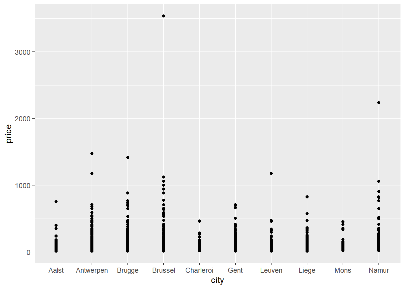
If all goes well, a plot should appear in the bottom right corner of your screen. Figures are made with the ggplot command. On the first line, you tell ggplot which data it should use to create a plot and which variables should appear on the X-axis and the Y-axis. We tell it to put city on the X-axis and price on the Y-axis. Specification of the X-axis and the Y-axis should always come as arguments to an aes function which itself is then provided as an argument to the mapping function. On the second line you tell ggplot to draw points (geom_point). When you are creating a plot, remember to always add a + at the end of each line of code that makes up the graph, except for the last one (adding the + at the beginning of a line won’t work).
The graph is not very informative because many points are drawn over each other.
2.6.2 Jitter
Let’s add jitter to our points:
ggplot(data = airbnb.topten, mapping = aes(x = city, y = price)) +
  geom_jitter() # Same code as before but now we replace geom_point with geom_jitter.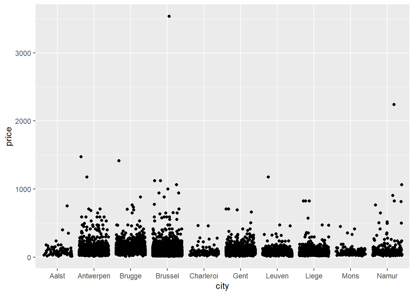
Instead of asking for points with geom_point(), we’ve now asked for points with added jitter with geom_jitter(). Jitter is a random value that gets added to each X and Y coordinate such that the data points are not drawn over each other. Note that we do this just to make the graph more informative (compare it to the previous scatterplot where many data points are drawn over each other); it does not change the actual values in our dataset.
2.6.3 Histogram
Still not clear though. It seems that the distribution of price is right-skewed. This means that the distribution of price is not normal. A normal distribution has two key features. A first feature is that there are more values close to the mean than there are values far away from the mean. In other words, extreme values don’t occur very often. A second feature is that the distribution is symmetrical. In other words, the number of values below the mean is equal to the number of values above the mean. In a skewed distribution, there are extreme outliers on only one side of the distribution. In case of right-skew, this means that there are extreme outliers on the right side of the distribution. In our case, this means that there are some Airbnb listings with very high prices. This inflates the mean of the distribution such that the listings are not normally distributed around the mean anymore.
Let’s draw a histogram of the prices:
ggplot(data = airbnb.topten, mapping = aes(x = price)) + # Notice that we don't have a x = city anymore. Price should be on the X-axis and the frequencies of the prices should be on the Y-axis
  geom_histogram() # Y-axis = frequency of values on X-axis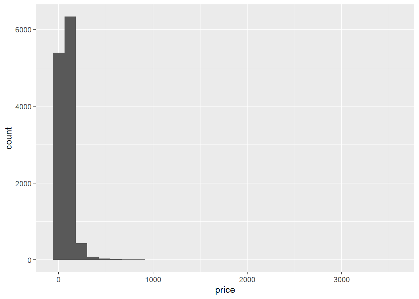
Indeed, there are some extremely high prices (compared to the majority of prices), so prices are right-skewed. Note: the stat_bin() using bins = 30. Pick better value with binwidth warning in the console can safely be ignored.
2.6.4 Log-transformation
Given that the price variable is right-skewed, we could log-transform it to make it more normal:
# On the Y-axis we now have log(price, base=exp(1)) instead of price. log(price, base=exp(1)) = take the natural logarithm, i.e., the logarithm with base = exp(1) = e.

ggplot(data = airbnb.topten, mapping = aes(x = city, y = log(price, base=exp(1)))) +
geom_jitter()![]()
2.6.5 Plot the median
Let’s get a better idea of the median price per city:
ggplot(data = airbnb.topten, mapping = aes(x = city, y = price)) +
  geom_jitter() +
  stat_summary(fun.y=median, colour="tomato3", size = 4, geom="point")
## Warning: The `fun.y` argument of `stat_summary()` is deprecated as of ggplot2 3.3.0.
## ℹ Please use the `fun` argument instead.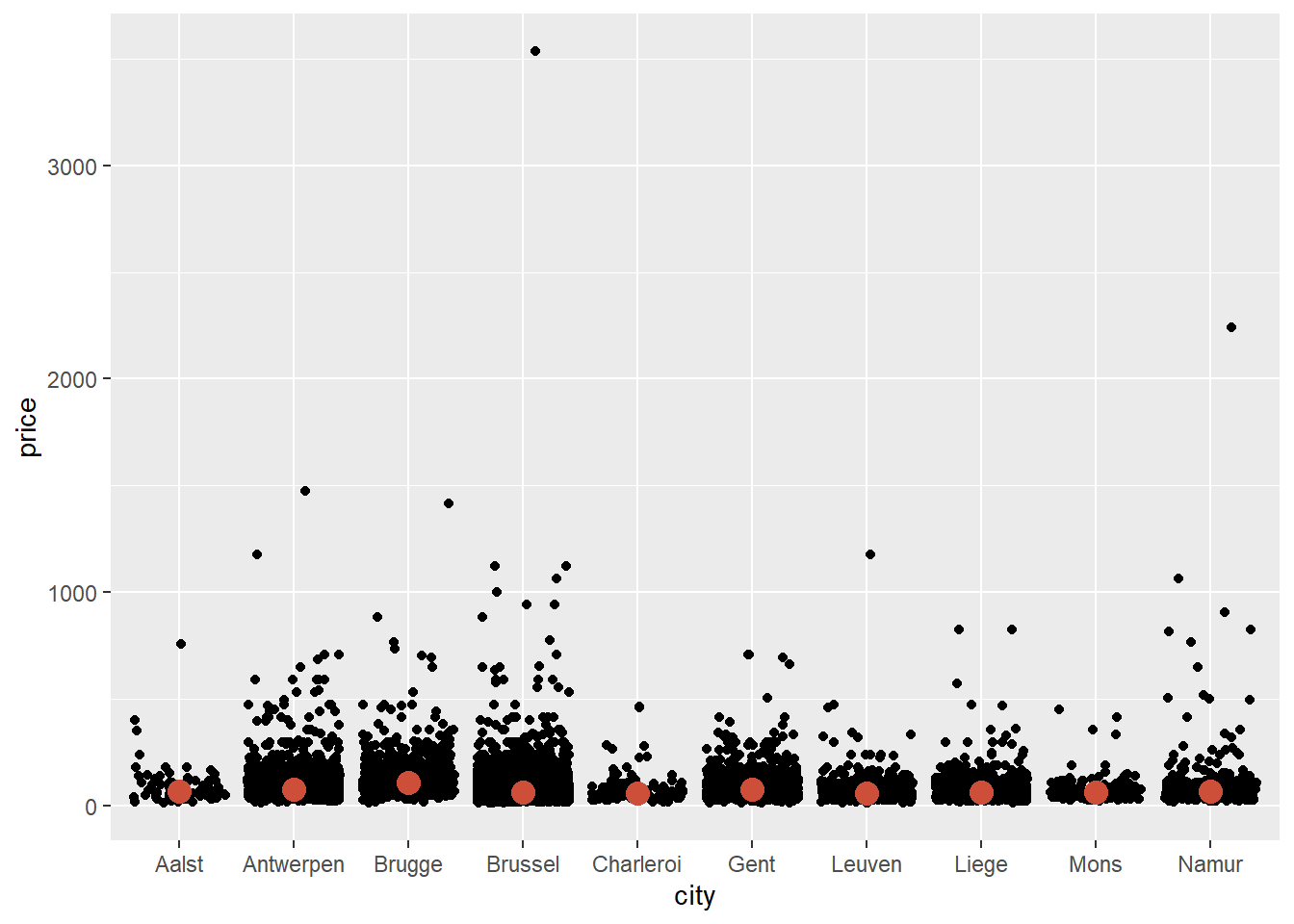
The line of code to get the median can be read as follows: stat_summary will ask for a statistical summary. The statistic we want is the median in a colour named "tomato3", with size 4. It should be represented as a "point".
We see that Brugge is the city with the highest median price. It’s much easier to see this when we log-transform price:
ggplot(data = airbnb.topten, mapping = aes(x = city, y = log(price, base = exp(1)))) +
  geom_jitter() +
  stat_summary(fun.y=median, colour="tomato3", size = 4, geom="point")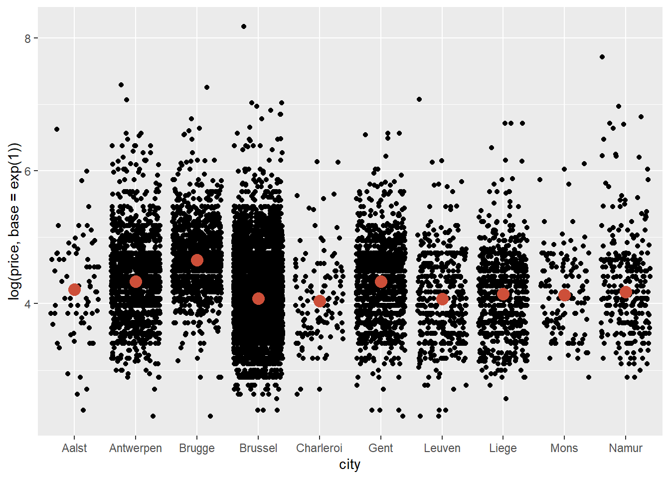
2.6.6 Plot the mean
Let’s add the mean as well, but in a different colour and shape than the mean:
ggplot(data = airbnb.topten, mapping = aes(x = city, y = log(price, base = exp(1)))) +
  geom_jitter() +
  stat_summary(fun.y=median, colour="tomato3", size = 4, geom="point") +
  stat_summary(fun.y=mean,   colour="green",   size = 4, geom="point", shape = 23, fill = "green")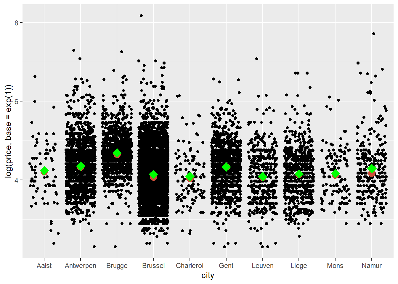
The code to obtain the mean is very similar to that used to obtain the median. We’ve simply changed the statistic, colour, and added shape = 23 to get diamonds instead of circles and fill = "green" to fill in the diamonds. We see that the means and medians are quite similar.
2.6.7 Saving images
We may want to save this plot on our hard drive. To do this click on Export/Save as Image. If you don’t change the directory, the file will be saved in your working directory. You can resize the plot and you should also give it a meaningful file name — Rplot01.png won’t be helpful when you try to find the file later.
A different (reproducible) way to save your file is to wrap the code in the png() and dev.off() functions:
png("price_per_city.png", width=800, height=600)
# This will prepare R to save the plot that will follow.
# Provide a filename and dimensions for the width and height of the picture in pixels.

ggplot(data = airbnb.topten, mapping = aes(x = city, log(price, base = exp(1)))) +
  geom_jitter() +
  stat_summary(fun.y=mean, colour="green", size = 4, geom="point", shape = 23, fill = "green") # I've only kept the mean here

dev.off() # This will tell R that we are done plotting and that it should save the plot to the hard drive.
Even though R has a non-graphical interface, it can create very nice graphs. Practically every little detail on the graph can be adjusted. Many of the graphs that you see in ‘data journalism’ (e.g., on https://www.nytimes.com/ or on http://fivethirtyeight.com/) are made in R.