4 Basic data analysis: experiments
In this chapter, we will analyze data from an experiment that tested whether people’s sense of power affects their willingness to pay (WTP) for status-related products (i.e., for conspicuous consumption) and whether this relationship is different when their WTP for these products is visible to others versus not.
Participants came to our lab in groups of eight or seven. They were seated in front of a computer in semi-closed cubicles. In the introduction, participants read that they would first have to fill in a personality questionnaire and a survey on how they dealt with money. After that, they would have to work together in groups of two on a few puzzles.
The first part of the session was a personality questionnaire assessing dominance and status aspirations (Cassidy & Lynn, 1989; Mead & Maner, 2012). Participants read 18 statements and indicated whether each of these statements applied to them or not. After completing this questionnaire, participants were reminded that at the end of the session they would have to work together with another participant on a few puzzles. Each dyad would consist of a manager and a worker. Participants read that assignment to these roles was based on their results on the personality questionnaire, but in reality, assignment to roles was random.
Participants in the high power condition then read that they were best suited to be manager whereas participants in the low power condition read that they were best suited to be worker (Galinsky, Gruenfeld, & Magee, 2003). The instructions made clear that managers would have more power in the puzzle-solving task than workers (they could decide how a potential bonus of 20 euros would be divided between manager and worker). Before starting the puzzles, however, participants were asked to first take part in a different study.
In an ostensibly different study, participants’ willingness to spend on conspicuous and inconspicuous products was measured. In the introduction to this part of the experiment, the presence of the audience was manipulated. In the private condition, participants were simply told that we were interested in their consumption patterns. They were asked how much they would spend on ten products that differed in the extent to which they could be used to signal status. The conspicuous or status-enhancing products were: a new car, a house, travels, clothes, and a wrist watch (for men) or jewelry (for women). The inconspicuous or status-neutral products were basic toiletries, household medication, a bedroom alarm clock, kitchen staples, and household cleaning (Griskevicius, et al., 2007). Participants responded on a nine-point scale ranging from 1: “I would buy very cheap items” to 9: “I would buy very expensive items”.
In the public condition, participants were told that we were working on a website where people could meet. This website would help us investigate how people form impressions of each other based on each other’s consumption patterns. Participants read that they would first have to indicate how much they would spend on a couple of products. Their choices would then be summarized in a profile. The other participants in the session would have to form impressions about them based on this profile. After viewing an example of what their profile could look like, participants moved on to the same consumption measure as in the private condition.
In short, the experiment has a 2 (power: high vs. low) x 2 (audience: public vs. private) x 2 (consumption: conspicuous vs. inconspicuous) design with power and audience manipulated between subjects and consumption manipulated within subjects.
The hypotheses in this experiment were as follows:
- In the private condition, we expected that low power participants would have a higher WTP than high power participants for conspicuous products but not for inconspicuous products. Such a pattern of results would replicate results from Rucker & Galinsky (2008).
- We expected that the public vs. private manipulation would lower WTP for conspicuous products for low power participants but not for high power participants. We did not expect an effect of the public vs. private manipulation on WTP for inconspicuous products for low nor high power participants.
This experiment is described in more detail in my doctoral dissertation (Franssens, 2016)
References:
Cassidy, T., & Lynn, R. (1989). A multifactorial approach to achievement motivation: The development of a comprehensive measure. Journal of Occupational Psychology, 62(4), 301-312.
Franssens, S. (2016). Essays in consumer behavior (Doctoral dissertation). KU Leuven, Leuven, Belgium.
Galinsky, A. D., Gruenfeld, D. H., & Magee, J. C. (2003). From Power to action. Journal of Personality and Social Psychology, 85(3), 453-466. https://doi.org/10.1037/0022-3514.85.3.453
Griskevicius, V., Tybur, J. M., Sundie, J. M., Cialdini, R. B., Miller, G. F., & Kenrick, D. T. (2007). Blatant benevolence and conspicuous consumption: When romantic motives elicit strategic costly signals. Journal of Personality and Social Psychology, 93(1), 85-102. https://doi.org/10.1037/0022-3514.93.1.85
Mead, N. L., & Maner, J. K. (2012). On keeping your enemies close: Powerful leaders seek proximity to ingroup power threats. Journal of Personality and Social Psychology, 102(3), 576-591. https://doi.org/10.1037/a0025755
Rucker, D. D., & Galinsky, A. D. (2008). Desire to acquire: Powerlessness and compensatory consumption. Journal of Consumer Research, 35(2), 257-267. https://doi.org/10.1086/588569
4.1 Data
4.1.1 Import
Download the data here. As always, save the data to a directory (preferably one that is automatically backed up by file-sharing software) and begin your script by loading the tidyverse and by setting the working directory to the directory where you have just saved your data:
library(tidyverse)
library(readxl) # we need this package because our data is stored in an Excel file
setwd("c:/dropbox/work/teaching/R/") # change to your own working directory

powercc <- read_excel("power_conspicuous_consumption.xlsx","data") # Import the Excel file. Note that the name of the Excel sheet is data
Don’t forget to save your script in the working directory.
4.1.2 Manipulate
powercc # Inspect the data## # A tibble: 147 × 39
## subject start_date end_date duration finished power audience group_size gender age
## <dbl> <dttm> <dttm> <dbl> <dbl> <chr> <chr> <dbl> <chr> <dbl>
## 1 1 2012-04-19 09:32:56 2012-04-19 09:49:42 1006. 1 high public 8 male 18
## 2 2 2012-04-19 09:31:26 2012-04-19 09:51:13 1187. 1 low public 8 male 18
## 3 3 2012-04-19 09:29:50 2012-04-19 09:53:10 1400. 1 low public 8 male 19
## 4 4 2012-04-19 09:26:25 2012-04-19 09:53:21 1616. 1 low public 8 male 18
## 5 5 2012-04-19 09:20:55 2012-04-19 09:54:21 2006. 1 high public 8 male 18
## 6 6 2012-04-19 09:28:02 2012-04-19 09:55:50 1668. 1 high public 8 male 20
## 7 7 2012-04-19 09:17:54 2012-04-19 09:58:49 2455. 1 low public 8 male 19
## 8 8 2012-04-19 09:22:26 2012-04-19 10:01:40 2354. 1 high public 8 male 19
## 9 9 2012-04-19 10:13:12 2012-04-19 10:31:03 1071. 1 low public 8 female 18
## 10 10 2012-04-19 10:12:55 2012-04-19 10:31:29 1114. 1 high public 8 female 18
## # … with 137 more rows, and 29 more variables: dominance1 <dbl>, dominance2 <dbl>, dominance3 <dbl>,
## # dominance4 <dbl>, dominance5 <dbl>, dominance6 <dbl>, dominance7 <dbl>, sa1 <dbl>, sa2 <dbl>,
## # sa3 <dbl>, sa4 <dbl>, sa5 <dbl>, sa6 <dbl>, sa7 <dbl>, sa8 <dbl>, sa9 <dbl>, sa10 <dbl>, sa11 <dbl>,
## # inconspicuous1 <dbl>, inconspicuous2 <dbl>, inconspicuous3 <dbl>, inconspicuous4 <dbl>,
## # inconspicuous5 <dbl>, conspicuous1 <dbl>, conspicuous2 <dbl>, conspicuous3 <dbl>, conspicuous4 <dbl>,
## # conspicuous5 <dbl>, agree <dbl>We have 39 columns or variables in our data:
subjectidentifies the participantsstart_dateandend_dateindicate the beginning and end of the experimental session.durationindicates the duration of the experimental sessionfinished: did participants complete the whole experiment?power(high vs. low) andaudience(private vs. public) are the experimental conditionsgroup_size: in groups of how many did participants come to the lab?genderandageof the participantdominance1,dominance2, etc. are the questions that measured dominance. An example is “I think I would enjoy having authority over other people”. Participants responded with yes (1) or no (0).sa1,sa2, etc. are the questions that measure status aspirations. An example is “I would like an important job where people looked up to me”. Participants responded with yes (1) or no (0).inconspicuous1,inconspicuous2, etc. contain the WTP for the inconspicuous products. Scale from 1: I would buy very cheap items to 9: I would buy very expensive items.conspicuous1,conspicuous2, etc. contain the WTP for the conspicuous products. Scale from 1: I would buy very cheap items to 9: I would buy very expensive items.agree: an exploratory question measuring whether people agreed they were better suited for the role of worker or manager. Participants responded on a scale from 1: much better suited for worker (manager) role to 7: much better suited for manager (worker) role. Higher numbers indicate agreement with the role assignment in the experiment.
4.1.2.1 Factorize some variables
Upon inspection of the data, we see that the type of subject is double, which means that subject should be factorized so that its values do not get treated as numbers. We’ll also factorize both our experimental conditions:
powercc <- powercc %>% # we've already created the powercc object before
  mutate(subject = factor(subject),
         power = factor(power, levels = c("low","high")), # note the levels argument
         audience = factor(audience, levels = c("private","public"))) # note the levels argument
Note that we’ve provided a new argument levels when factorizing power and audience. This argument specifies the order of the levels of a factor. In the context of this experiment, it is more natural to talk about the effect of high vs. low power on consumption than to talk about the effect of low vs. high power on consumption. Therefore, we tell R that the low power level should be considered as the first level. Later on we’ll see that the output of analyses can then be interpreted as effects of high power (second level) vs. low power (first level). The same reasoning applies to the audience factor, although providing the levels for this factor was unnecessary because private comes before public alphabetically. Your choice of level for the first or reference level only influences interpretation, not the actual outcome of the analysis.
In one experimental session, the fire alarm went off and we had to leave the lab. Let’s remove participants who did not complete the experiment:
powercc <- powercc %>% # we've already created the powercc object before
  filter(finished == 1) # only retain observations where finished is equal to 1
Notice the double == when testing for equality. Check out the R 4 Data Science book for other logical operators (scroll down to get to Section 5.2.2).
4.1.2.2 Calculate the internal consistency & the average of questions that measure the same concept
We would like to average the questions that measure dominance to get a single number indicating whether the participant has a dominant or a non-dominant personality. Before we do this, we should get an idea of the internal consistency of the questions that measure dominance. This will tell us whether all these questions measure the same concept. One measure of internal consistency is Cronbach’s alpha. To calculate it, we need a package called psych:
install.packages("psych")
library(psych)
Once this package is loaded, we can use the alpha function to calculate Cronbach’s alpha for a set of questions:
dominance.questions <- powercc %>%
  select(starts_with("dominance")) # take the powercc data frame and select all the variables with a name that starts with dominance

alpha(dominance.questions) # calculate the cronbach alpha of these variables
##
## Reliability analysis
## Call: alpha(x = dominance.questions)
##
## raw_alpha std.alpha G6(smc) average_r S/N ase mean sd median_r
## 0.69 0.67 0.67 0.23 2.1 0.038 0.63 0.27 0.21
##
## 95% confidence boundaries
## lower alpha upper
## Feldt 0.60 0.69 0.76
## Duhachek 0.61 0.69 0.76
##
## Reliability if an item is dropped:
## raw_alpha std.alpha G6(smc) average_r S/N alpha se var.r med.r
## dominance1 0.68 0.67 0.66 0.25 2.0 0.039 0.016 0.22
## dominance2 0.65 0.63 0.62 0.22 1.7 0.043 0.018 0.21
## dominance3 0.59 0.58 0.56 0.19 1.4 0.050 0.014 0.20
## dominance4 0.62 0.60 0.59 0.20 1.5 0.047 0.018 0.21
## dominance5 0.65 0.64 0.63 0.23 1.7 0.043 0.021 0.21
## dominance6 0.70 0.70 0.68 0.28 2.4 0.038 0.009 0.25
## dominance7 0.65 0.64 0.62 0.23 1.8 0.043 0.017 0.20
##
## Item statistics
## n raw.r std.r r.cor r.drop mean sd
## dominance1 143 0.52 0.49 0.33 0.29 0.53 0.50
## dominance2 143 0.59 0.61 0.52 0.42 0.80 0.40
## dominance3 143 0.75 0.74 0.71 0.59 0.52 0.50
## dominance4 143 0.68 0.68 0.61 0.50 0.58 0.50
## dominance5 143 0.61 0.59 0.48 0.40 0.55 0.50
## dominance6 143 0.29 0.38 0.19 0.14 0.91 0.29
## dominance7 143 0.62 0.59 0.48 0.41 0.53 0.50
##
## Non missing response frequency for each item
## 0 1 miss
## dominance1 0.47 0.53 0
## dominance2 0.20 0.80 0
## dominance3 0.48 0.52 0
## dominance4 0.42 0.58 0
## dominance5 0.45 0.55 0
## dominance6 0.09 0.91 0
## dominance7 0.47 0.53 0# Note that we could have also written this as follows:
# powercc %>% select(starts_with("dominance")) %>% cronbach()This produces a lot of output. Under raw_alpha, we see that the alpha is 0.69, which is on the lower side (.70 is often considered the minimum required), but still ok. The table below tells us what the alpha would be if we dropped one question from our measure. Dropping dominance6 would increase the alpha to 0.7. Compared to the original alpha of 0.69, this increase is tiny and hence we don’t drop dominance6. If there were a question with a high ‘alpha if dropped’, then this would indicate that this question is measuring something different than the other questions. In that case, you could consider removing this question from your measure.
We can proceed by averaging the responses on the dominance question:
powercc <- powercc %>%
  mutate(dominance = (dominance1+dominance2+dominance3+dominance4+dominance5+dominance6+dominance7)/7,
         cc = (conspicuous1+conspicuous2+conspicuous3+conspicuous4+conspicuous5)/5,
         icc = (inconspicuous1+inconspicuous2+inconspicuous3+inconspicuous4+inconspicuous5)/5) %>%
  select(-starts_with("sa"))
I’ve also averaged the questions about conspicuous consumption and inconspicuous consumption, but not the questions about status aspirations because their Cronbach alpha was too low. I’ve deleted the questions about status aspirations from the dataset. I leave it as an exercise to check the Cronbach alpha’s of each of these concepts (do this before deleting the questions about status aspirations, of course).
4.1.3 Recap: importing & manipulating
Here’s what we’ve done so far, in one orderly sequence of piped operations (download the data here):
library(tidyverse)
library(readxl)
setwd("c:/dropbox/work/teaching/R/") # change to your own working directory

powercc <- read_excel("power_conspicuous_consumption.xlsx","data")  %>%
  filter(finished == 1) %>%
  mutate(subject = factor(subject),
         power = factor(power, levels = c("low","high")),
         audience = factor(audience, levels = c("private","public")),
         dominance = (dominance1+dominance2+dominance3+dominance4+dominance5+dominance6+dominance7)/7,
         cc = (conspicuous1+conspicuous2+conspicuous3+conspicuous4+conspicuous5)/5,
         icc = (inconspicuous1+inconspicuous2+inconspicuous3+inconspicuous4+inconspicuous5)/5) %>%
  select(-starts_with("sa"))
4.2 t-tests
4.2.1 Independent samples t-test
Say we want to test whether men and women differ in the degree to which they are dominant. Let’s create a boxplot first and then check the means and the standard deviations:
ggplot(data = powercc, mapping = aes(x = gender, y = dominance)) +
  geom_boxplot()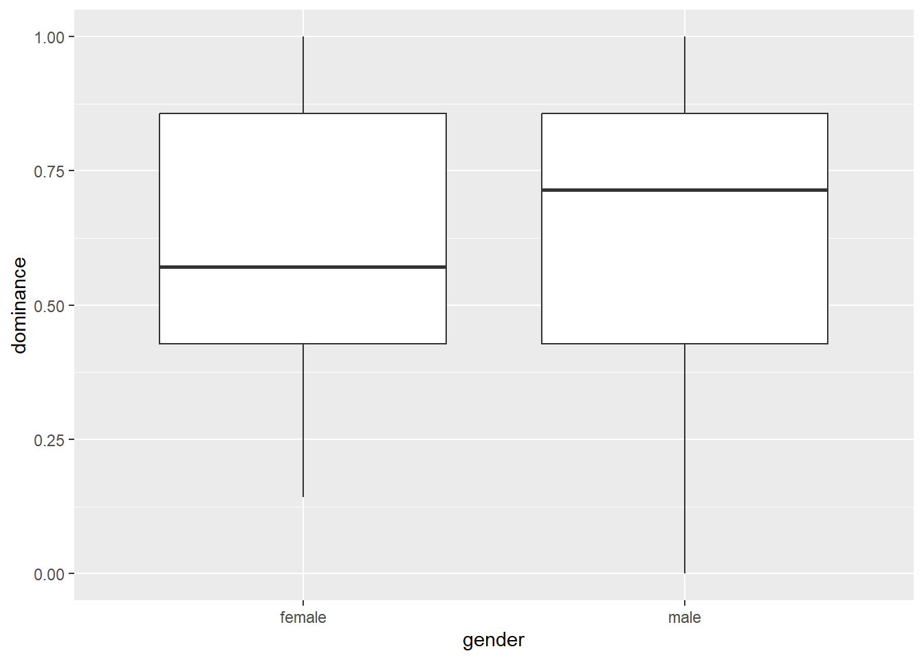
powercc %>%
  group_by(gender) %>%
  summarize(mean_dominance = mean(dominance),
            sd_dominance = sd(dominance))
## # A tibble: 2 × 3
## gender mean_dominance sd_dominance
## <chr> <dbl> <dbl>
## 1 female 0.614 0.247
## 2 male 0.646 0.296Men score slightly higher than women, but we want to know whether this difference is significant. An independent samples t-test can provide the answer (the men and the women in our experiment are the independent samples), but we need to check an assumption first: are the variances of the two independent samples equal?
install.packages("car") # for the test of equal variances, we need a package called car
library(car)
# Levene's test of equal variances.
# Low p-value means the variances are not equal.
# First argument = continuous dependent variable, second argument = categorical independent variable.
leveneTest(powercc$dominance, powercc$gender) ## Levene's Test for Homogeneity of Variance (center = median)
## Df F value Pr(>F)
## group 1 2.1915 0.141
## 141The null hypothesis of equal variances is not rejected (p = 0.14), so we can continue with a t-test that assumes equal variances:
# Test whether the means of dominance differ between genders.
# Indicate whether the test should assume equal variances or not (set var.equal = FALSE for a test that does not assume equal variances).
t.test(powercc$dominance ~ powercc$gender, var.equal = TRUE)
##
## Two Sample t-test
##
## data: powercc$dominance by powercc$gender
## t = -0.6899, df = 141, p-value = 0.4914
## alternative hypothesis: true difference in means between group female and group male is not equal to 0
## 95 percent confidence interval:
## -0.12179092 0.05877722
## sample estimates:
## mean in group female mean in group male
## 0.6142857 0.6457926You could report this as follows: “Men (M = 0.65, SD = 0.3) and women (M = 0.61, SD = 0.25) did not differ in the degree to which they rated themselves as dominant (t(141) = -0.69, p = 0.49).”
4.2.2 Dependent samples t-test
Say we want to test whether people are more willing to spend on conspicuous items than on inconspicuous items. Let’s check the means and the standard deviations first:
powercc %>% # no need to group! we're not splitting up our sample into subgroups
  summarize(mean_cc = mean(cc), sd_cc = sd(cc),
            mean_icc = mean(icc), sd_icc = sd(icc))
## # A tibble: 1 × 4
## mean_cc sd_cc mean_icc sd_icc
## <dbl> <dbl> <dbl> <dbl>
## 1 6.01 1.05 3.60 0.988The means are higher for conspicuous products than for inconspicuous products, but we want to know whether this difference is significant and therefore perform a dependent samples t-test (each participant rates both conspicuous and inconspicuous products, so these ratings are dependent):
t.test(powercc$cc, powercc$icc, paired = TRUE) # Test whether the means of cc and icc are different. Indicate that this is a dependent samples t-test with paired = TRUE.##
## Paired t-test
##
## data: powercc$cc and powercc$icc
## t = 25.064, df = 142, p-value < 2.2e-16
## alternative hypothesis: true mean difference is not equal to 0
## 95 percent confidence interval:
## 2.214575 2.593816
## sample estimates:
## mean difference
## 2.404196You could report this as follows: “People indicated they were willing to pay more (t(142) = 25.064, p < .001) for conspicuous products (M = 6.01, SD = 1.05) than for inconspicuous products (M = 3.6, SD = 0.99).”
4.2.3 One sample t-test
Say we want to test whether the average willingness to pay for the conspicuous items was significantly higher than 5 (the midpoint of the scale):
t.test(powercc$cc, mu = 5) # Indicate the variable whose mean we want to compare with a specific value (5).##
## One Sample t-test
##
## data: powercc$cc
## t = 11.499, df = 142, p-value < 2.2e-16
## alternative hypothesis: true mean is not equal to 5
## 95 percent confidence interval:
## 5.833886 6.180100
## sample estimates:
## mean of x
## 6.006993It’s indeed significantly higher than 5. You could report this as follows: “The average WTP for conspicuous products (M = 6.01, SD = 1.05) was significantly above 5 (t(142) = 11.499, p < .001).”
4.3 Two-way ANOVA
When you read an academic paper that reports an experiment, the results section often starts with a discussion of the main effects of the experimental factors and their interaction, as tested by an Analysis of Variance or ANOVA. Let’s focus on WTP for status-enhancing products first. (We have briefly considered the WTP for status-neutral products in our discussion of dependent samples t-tests and we’ll discuss it in more detail in the section on repeated measures ANOVA.)
Let’s inspect some descriptive statistics first. We’d like to view the mean WTP for conspicuous products, the standard deviation of this WTP, and the number of participants in each experimental cell. We’ve already learned how to do some of this in the introductory chapter (see frequency tables and descriptive statistics):
powercc.summary <- powercc %>% # we're assigning the summary to an object, because we'll need this summary to make a bar plot
  group_by(audience, power) %>% # we now group by two variables!
  summarize(count = n(),
            mean = mean(cc),
            sd = sd(cc))
## `summarise()` has grouped output by 'audience'. You can override using the `.groups` argument.powercc.summary## # A tibble: 4 × 5
## # Groups: audience [2]
## audience power count mean sd
## <fct> <fct> <int> <dbl> <dbl>
## 1 private low 34 6.08 1.04
## 2 private high 31 5.63 0.893
## 3 public low 40 6.17 1.15
## 4 public high 38 6.07 1.03We see that the difference in WTP between high and low power participants is larger in the private than in the public condition.
Let’s summarize these results in a box plot:
# when creating a box plot, the dataset that serves as input to ggplot is the full dataset, not the summary with the means
ggplot(data = powercc, mapping = aes(x = audience, y = cc, fill = power)) +
  geom_boxplot() # arguments are the same as for geom_bar, but now we provide them to geom_boxplot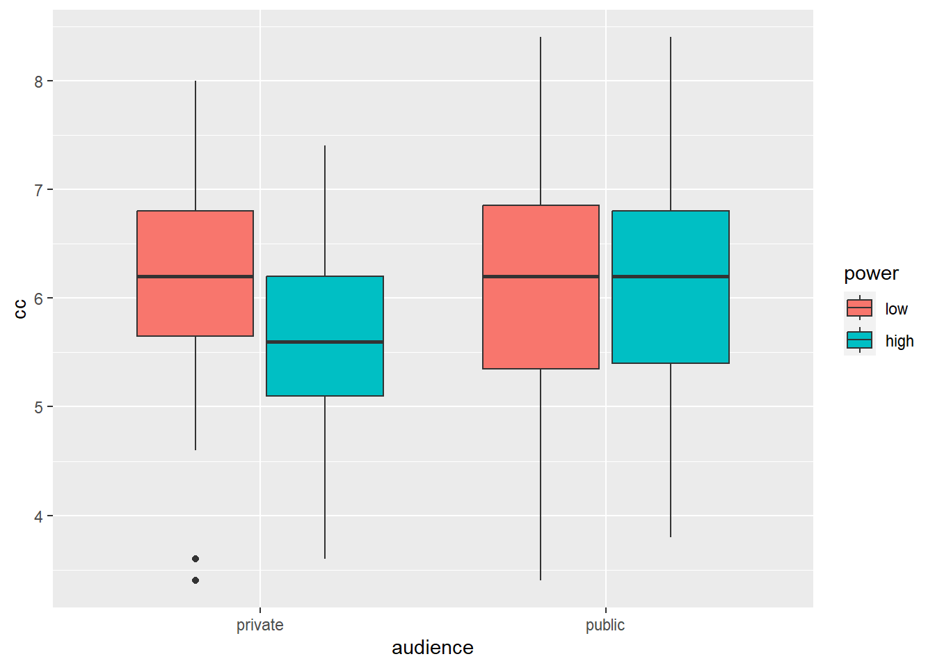
Box plots are informative because they give us an idea of the median and of the distribution of the data. However, in academic papers, the results of experiments are traditionally summarized in bar plots (even though boxplots are more informative).
 # when creating a bar plot, the dataset that serves as input to ggplot is the summary with the means, not the full dataset
ggplot(data = powercc.summary, mapping = aes(x = audience, y = mean, fill = power)) +
  geom_bar(stat = "identity", position = "dodge")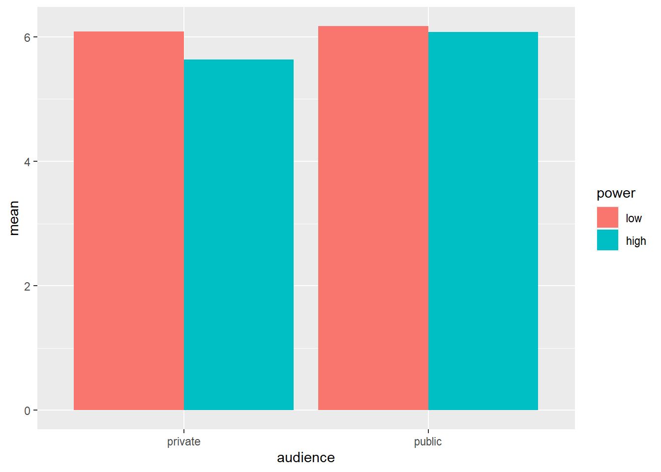
To create a bar plot, we tell ggplot the variables that should be on the X-axis and the Y-axis and we also tell it to use different colors for different levels of power with the fill command. Then we ask for a bar plot with geom_bar. stat = "identity" and position = "dodge" should be included as arguments for geom_bar, but a discussion of these arguments is beyond the scope of this tutorial.
Before we proceed with the ANOVA, we should check whether its assumptions are met. We’ve discussed the assumptions of ANOVA previously, but we skip checking it here.
To carry out an ANOVA, we need to install some packages:
install.packages("remotes") # The remotes package allows us to install packages that are stored on GitHub, a website for package developers.
install.packages("car") # We'll need the car package as well to carry out the ANOVA (no need to re-install this if you have done this already).

library(remotes)
install_github('samuelfranssens/type3anova') # Install the type3anova package. This and the previous steps need to be carried out only once.

library(type3anova) # Load the type3anova package.
We can now proceed with the actual ANOVA:
# First create a linear model
# The lm() function takes a formula and a data argument
# The formula has the following syntax: dependent variable ~ independent variable(s)
linearmodel <- lm(cc ~ power*audience, data=powercc)
# power*audience: interaction is included
# power+audience: interaction is not included

type3anova(linearmodel) # Then ask for output in ANOVA format. This gives Type III sum of squares. Note that this is different from anova(linearmodel) which gives Type I sum of squares.
## # A tibble: 5 × 6
## term ss df1 df2 f pvalue
## <chr> <dbl> <dbl> <int> <dbl> <dbl>
## 1 (Intercept) 5080. 1 139 4710. 0
## 2 power 2.64 1 139 2.45 0.12
## 3 audience 2.48 1 139 2.30 0.132
## 4 power:audience 1.11 1 139 1.03 0.313
## 5 Residuals 150. 139 139 NA NAYou could report these results as follows: “Neither the main effect of power (F(1, 139) = 2.45, p = 0.12), nor the main effect of audience (F(1, 139) = 2.3, p = 0.13), nor the interaction between power and audience (F(1, 139) = 1.03, p = 0.31) was significant.”
4.3.1 Following up with contrasts
When carrying out a 2 x 2 experiment, we’re often hypothesizing an interaction. An interaction means that the effect of one independent variable is different depending on the levels of the other independent variable. In the previous section, the ANOVA told us that the interaction between power and audience was not significant. This means that the effect of high vs. low power was the same in the private and in the public condition and that the effect of public vs. private was the same in the high and in the low power condition. Normally, the analysis would stop with the non-significance of the interaction. However, we’re going to carry out the follow-up tests that one would do if the interaction were significant.
Let’s consider the cell means again:
powercc.summary <- powercc %>%
  group_by(audience, power) %>%
  summarize(count = n(),
            mean = mean(cc),
            sd = sd(cc))
## `summarise()` has grouped output by 'audience'. You can override using the `.groups` argument.# when creating a bar plot, the dataset that serves as input to ggplot is the summary with the means, not the full dataset
ggplot(data = powercc.summary,mapping = aes(x = audience, y = mean, fill = power)) +
geom_bar(stat = "identity", position = "dodge")
powercc.summary## # A tibble: 4 × 5
## # Groups: audience [2]
## audience power count mean sd
## <fct> <fct> <int> <dbl> <dbl>
## 1 private low 34 6.08 1.04
## 2 private high 31 5.63 0.893
## 3 public low 40 6.17 1.15
## 4 public high 38 6.07 1.03We want to test whether the difference between high and low power within the private condition is significant (low: 6.08 vs. high: 5.63) and whether the difference between high and low power within the public condition is significant (low: 6.17 vs. high: 6.07). To do this, we can use the contrast function from the type3anova library that we’ve installed previously. The contrast function takes two arguments: a linear model and a contrast specification. The linear model is the same as before:
linearmodel <- lm(cc ~ power*audience, data=powercc)But to know how we should specify our contrast, we need to take a look at the regression coefficients in our linear model:
summary(linearmodel)##
## Call:
## lm(formula = cc ~ power * audience, data = powercc)
##
## Residuals:
## Min 1Q Median 3Q Max
## -2.7700 -0.6737 0.1177 0.7177 2.3263
##
## Coefficients:
## Estimate Std. Error t value Pr(>|t|)
## (Intercept) 6.08235 0.17812 34.148 <2e-16 ***
## powerhigh -0.45009 0.25792 -1.745 0.0832 .
## audiencepublic 0.08765 0.24226 0.362 0.7181
## powerhigh:audiencepublic 0.35378 0.34910 1.013 0.3126
## ---
## Signif. codes: 0 '***' 0.001 '**' 0.01 '*' 0.05 '.' 0.1 ' ' 1
##
## Residual standard error: 1.039 on 139 degrees of freedom
## Multiple R-squared: 0.03711, Adjusted R-squared: 0.01633
## F-statistic: 1.786 on 3 and 139 DF, p-value: 0.1527We have four regression coefficients:
- \(\beta_0\) or the intercept (6.08)
- \(\beta_1\) or the coefficient for “powerhigh”, or the high level of the power factor (-0.45)
- \(\beta_2\) or the coefficient for “audiencepublic”, or the public level of the audience factor (0.09)
- \(\beta_3\) or the coefficient for “powerhigh:audiencepublic” (0.35)
We see that the estimate for the intercept corresponds to the observed mean in the low power, private cell. Add to this the estimate of “powerhigh” and one gets the observed mean in the high power, private cell. Add to the estimate for the intercept, the estimate of “audiencepublic” and one gets the observed mean in the low power, public cell. Add to the estimate for the intercept, the estimate of “powerhigh”, “audiencepublic”, and “powerhigh:audiencepublic” and one gets the observed mean in the high power, public cell. I usually visualize this in a table (and save this in my script) to make it easier to specify the contrast I want to test:
#                   private             public
# low power         b0                  b0+b2
# high power        b0+b1               b0+b1+b2+b3
Say we’re contrasting high vs. low power in the private condition, then we’re testing whether (\(\beta_0\) + \(\beta_1\)) and \(\beta_0\) differ significantly, or whether (\(\beta_0\) + \(\beta_1\)) - \(\beta_0\) = \(\beta_1\) is significantly different from zero. We specify this as follows:
contrast_specification <- c(0, 1, 0, 0)
# the four numbers correspond to b0, b1, b2, b3.
# we want to test whether b1 is significant, so we put a 1 in 2nd place (1st place is for b0)

contrast(linearmodel, contrast_specification)
##
## Simultaneous Tests for General Linear Hypotheses
##
## Fit: aov(formula = linearmodel)
##
## Linear Hypotheses:
## Estimate Std. Error t value Pr(>|t|)
## 1 == 0 -0.4501 0.2579 -1.745 0.0832 .
## ---
## Signif. codes: 0 '***' 0.001 '**' 0.01 '*' 0.05 '.' 0.1 ' ' 1
## (Adjusted p values reported -- single-step method)The output tells us the estimate of the contrast is -0.45, which is indeed the difference between the observed means in the private condition (high power: 5.63 vs. low power: 6.08). You could report this result as follows: “The effect of high (M = 5.63, SD = 0.89) vs. low power (M = 6.08, SD = 1.04) in the private condition was marginally significant (t(139) = -1.745, p = 0.083).” To get the degrees of freedom, do contrast(linearmodel, contrast_specification)$df.
Say we want to test a more complicated contrast, namely whether the mean in the high power, private cell is different from the average of the means in the other cells. We’re testing:
(\(\beta_0\) + \(\beta_1\)) - 1/3 * [(\(\beta_0\)) + (\(\beta_0\) + \(\beta_2\)) + (\(\beta_0\) + \(\beta_1\) + \(\beta_2\) + \(\beta_3\))]
= \(\beta_1\) - 1/3 * (\(\beta_1\) + 2*\(\beta_2\) + \(\beta_3\))
= 2/3 \(\beta_1\) - 2/3 \(\beta_2\) - 1/3 \(\beta_3\)
The contrast specification is as follows:
contrast_specification <- c(0, 2/3, -2/3, -1/3)
contrast(linearmodel, contrast_specification)
##
## Simultaneous Tests for General Linear Hypotheses
##
## Fit: aov(formula = linearmodel)
##
## Linear Hypotheses:
## Estimate Std. Error t value Pr(>|t|)
## 1 == 0 -0.4764 0.2109 -2.259 0.0254 *
## ---
## Signif. codes: 0 '***' 0.001 '**' 0.01 '*' 0.05 '.' 0.1 ' ' 1
## (Adjusted p values reported -- single-step method)Check whether the estimate indeed corresponds to the difference between the mean of high power, private and the average of the means in the other cells. You could report this as follows: “The high power, private cell had a significantly lower WTP than the other experimental cells in our design (est = -0.476, t(139) = -2.259, p = 0.025)”.
4.4 Moderation analysis: Interaction between continuous and categorical independent variables
Say we want to test whether the results of the experiment depend on people’s level of dominance. In other words, are the effects of power and audience different for dominant vs. non-dominant participants? In still other words, is there a three-way interaction between power, audience, and dominance?
Let’s create a graph first:
# Our dependent variable is conspicuous consumption, our independent variable (on the X-axis) is dominance.
# So we're plotting the relationship between dominance and conspicuous consumption.
# The color argument tells R that we want a relationship for each level of power.

ggplot(data = powercc, mapping = aes(x = dominance, y = cc, color = power)) +
  facet_wrap(~ audience) + # Tell R that we also want to split up by audience.
  geom_jitter() + # Use geom_jitter instead of geom_point, otherwise the points are drawn over each other
  geom_smooth(method='lm', se=FALSE) # Draw a linear regression line through the points.
## `geom_smooth()` using formula = 'y ~ x'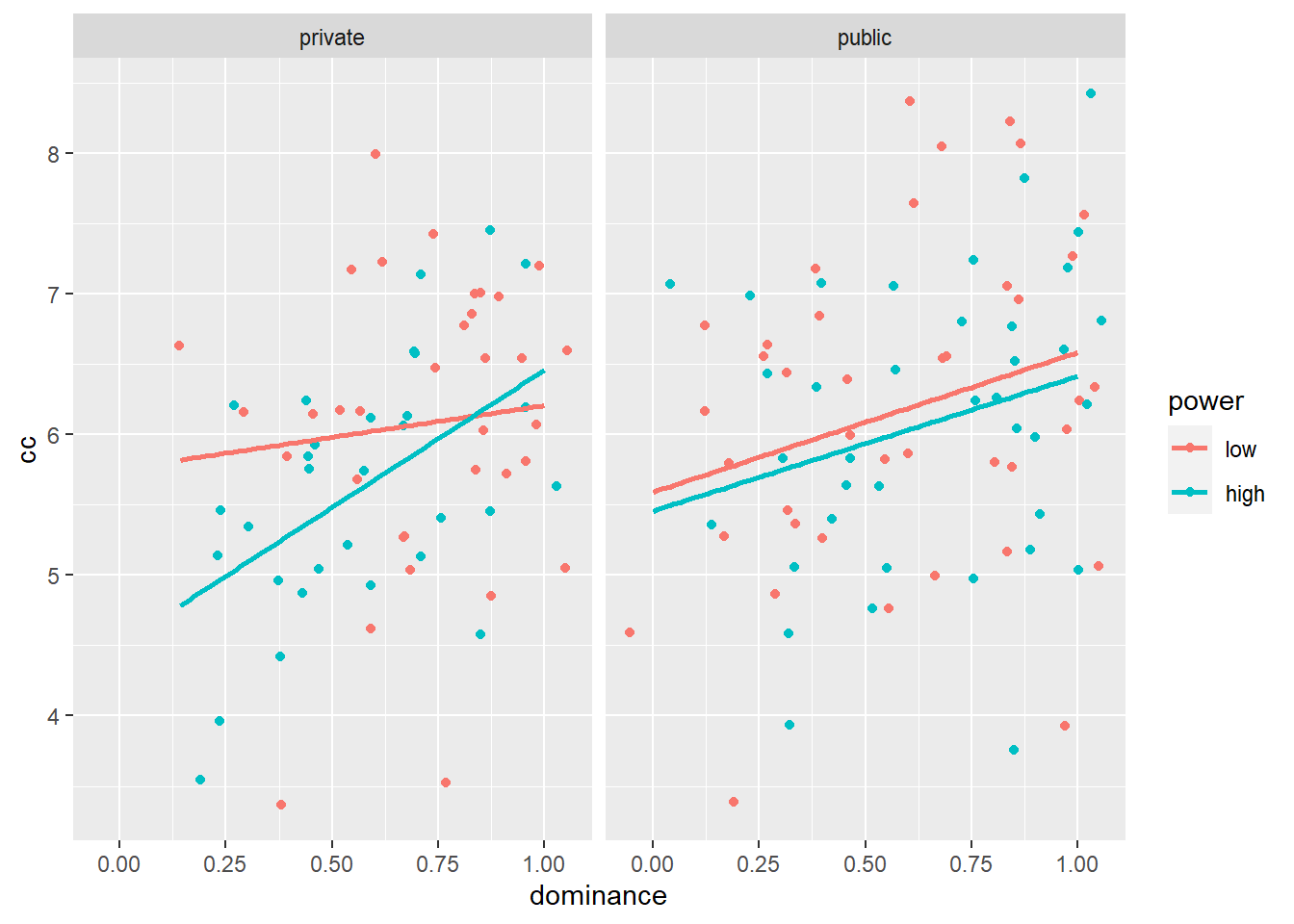
This graph is informative. It shows us that in the private condition, the effect of high vs. low power on conspicuous consumption is more negative for less dominant participants than for more dominant participants. In the public condition, the effect of high vs. low power on conspicuous consumption does not differ between less vs. more dominant participants. We also see that in both the private and the public condition, more vs. less dominant participants are more willing to spend on conspicuous consumption.
Let’s check whether the three-way interaction is significant:
linearmodel <- lm(cc ~ power * audience * dominance, data = powercc)
type3anova(linearmodel)
## # A tibble: 9 × 6
## term ss df1 df2 f pvalue
## <chr> <dbl> <dbl> <int> <dbl> <dbl>
## 1 (Intercept) 525. 1 135 519. 0
## 2 power 2.21 1 135 2.18 0.142
## 3 audience 0.715 1 135 0.706 0.402
## 4 dominance 10.5 1 135 10.3 0.002
## 5 power:audience 1.44 1 135 1.42 0.235
## 6 power:dominance 1.18 1 135 1.17 0.282
## 7 audience:dominance 0.113 1 135 0.111 0.739
## 8 power:audience:dominance 1.30 1 135 1.29 0.258
## 9 Residuals 137. 135 135 NA NAOnly the effect of dominance is significant. If the three-way interaction were significant, we could follow-up with more tests. For example, we could test whether the two-way interaction between dominance and power is significant in the private condition, as the graph suggests. To do this, let’s first take a look at the regression coefficients of our linear model:
summary(linearmodel)##
## Call:
## lm(formula = cc ~ power * audience * dominance, data = powercc)
##
## Residuals:
## Min 1Q Median 3Q Max
## -2.58617 -0.63357 0.09751 0.68310 2.24067
##
## Coefficients:
## Estimate Std. Error t value Pr(>|t|)
## (Intercept) 5.7553 0.6019 9.561 <2e-16 ***
## powerhigh -1.2490 0.7703 -1.621 0.107
## audiencepublic -0.1651 0.6918 -0.239 0.812
## dominance 0.4526 0.7980 0.567 0.572
## powerhigh:audiencepublic 1.1162 0.9355 1.193 0.235
## powerhigh:dominance 1.5021 1.1111 1.352 0.179
## audiencepublic:dominance 0.5434 0.9514 0.571 0.569
## powerhigh:audiencepublic:dominance -1.5394 1.3561 -1.135 0.258
## ---
## Signif. codes: 0 '***' 0.001 '**' 0.01 '*' 0.05 '.' 0.1 ' ' 1
##
## Residual standard error: 1.006 on 135 degrees of freedom
## Multiple R-squared: 0.1225, Adjusted R-squared: 0.07703
## F-statistic: 2.693 on 7 and 135 DF, p-value: 0.01211We have eight terms in our model:
- \(\beta_0\) or the intercept
- \(\beta_1\) or the coefficient for “powerhigh”
- \(\beta_2\) or the coefficient for “audiencepublic”
- \(\beta_3\) or the coefficient for “dominance”
- \(\beta_4\) or the coefficient for “powerhigh:audiencepublic”
- \(\beta_5\) or the coefficient for “powerhigh:dominance”
- \(\beta_6\) or the coefficient for “audiencepublic:dominance”
- \(\beta_7\) or the coefficient for “powerhigh:audiencepublic:dominance”
Resulting in this table of coefficients:
#                     private                         public
# low power          [b0] + (b3)                     [b0+b2] + (b3+b6)
# high power         [b0+b1] + (b3+b5)               [b0+b1+b2+b4] + (b3+b5+b6+b7)
How did we get this table? With the linear model specified above, each estimated value of conspicuous consumption (the dependent variable) is a function the participant’s experimental condition and the participant’s level of dominance. Say we have a participant in the low power, public condition with a level of dominance of 0.5. The estimated value of conspicuous consumption for this participant is:
- \(\beta_0\): intercept \(\times\) 1
- \(\beta_1\): “powerhigh” \(\times\) 0 (because the participant is not in the high power condition)
- \(\beta_2\): “audiencepublic” \(\times\) 1 (in the public condition)
- \(\beta_3\): “dominance” \(\times\) 0.5 (dominance = 0.5)
- \(\beta_4\): “powerhigh:audiencepublic” \(\times\) 0 (not in both the high power & the public condition)
- \(\beta_5\): “powerhigh:dominance” \(\times\) 0 (not in the high power condition)
- \(\beta_6\): “audiencepublic:dominance” \(\times\) 1 \(\times\) 0.5 (in the public condition and dominance = 0.5)
- \(\beta_7\): “powerhigh:audiencepublic:dominance” \(\times\) 0 (not in both the high power & the public condition)
or \(\beta_0\) \(\times\) 1 + \(\beta_1\) \(\times\) 0 + \(\beta_2\) \(\times\) 1 + \(\beta_3\) \(\times\) 0.5 + \(\beta_4\) \(\times\) 0 + \(\beta_5\) \(\times\) 0 + \(\beta_6\) \(\times\) 0.5 + \(\beta_7\) \(\times\) 0
= [\(\beta_0\) + \(\beta_2\)] + (\(\beta_3\) + \(\beta_6\)) \(\times\) 0.5
= [5.76 + -0.17] + (0.45 + 0.54) * 0.5 = 6.09
Check the graph to see that this indeed corresponds to the estimated conspicuous consumption of a participant with dominance = 0.5 in the low power, public cell.
The general formula for the low power, public cell is the following:
[\(\beta_0\) + \(\beta_2\)] + (\(\beta_3\) + \(\beta_6\)) \(\times\) dominance
and we can obtain the formulas for the different cells in a similar manner. We see that in each cell, the coefficient between square brackets is the estimated value on the conspicuous consumption measure for a participant who scores 0 on dominance. The coefficient between round brackets is the estimated increase in the conspicuous consumption measure for every one unit increase in dominance. In other words, the coefficients between square brackets represent the intercept and the coefficients between round brackets represent the slope of the line that represents the regression of conspicuous consumption (Y) on dominance (X) within each experimental cell (i.e., each power & audience combination).
A test of the interaction between power and dominance within the private condition would come down to testing whether the blue and the red line in the left panel of the figure above should be considered parallel or not. If they are parallel, then the effect of dominance on conspicuous consumption is the same in the low and the high power condition. If they’re not parallel, then the effect of dominance is different in the low versus the high power condition. In other words, we should test whether the regression coefficients are equal within low power, private and within high power, private. In still other words, we test whether (\(\beta_3\) + \(\beta_5\)) - \(\beta_3\) = \(\beta_5\) is equal to zero:
# now we have eight numbers corresponding to the eight regression coefficients
# we want to test whether b5 is significant, so we put a 1 in 6th place (1st place is for b0)
contrast_specification <- c(0, 0, 0, 0, 0, 1, 0, 0)

contrast(linearmodel, contrast_specification)
##
## Simultaneous Tests for General Linear Hypotheses
##
## Fit: aov(formula = linearmodel)
##
## Linear Hypotheses:
## Estimate Std. Error t value Pr(>|t|)
## 1 == 0 1.502 1.111 1.352 0.179
## (Adjusted p values reported -- single-step method)The interaction is not significant, however. You could report this as follows: “Within the private condition, there was no interaction between power and dominance (t(135) = 1.352, p = 0.18).”
4.5 ANCOVA
We’ve found that our experimental conditions do not significantly affect conspicuous consumption:
linearmodel1 <- lm(cc ~ power*audience, data = powercc)
type3anova(linearmodel1)
## # A tibble: 5 × 6
## term ss df1 df2 f pvalue
## <chr> <dbl> <dbl> <int> <dbl> <dbl>
## 1 (Intercept) 5080. 1 139 4710. 0
## 2 power 2.64 1 139 2.45 0.12
## 3 audience 2.48 1 139 2.30 0.132
## 4 power:audience 1.11 1 139 1.03 0.313
## 5 Residuals 150. 139 139 NA NAOn the one hand, this could mean that there simply are no effects of the experimental conditions on conspicuous consumption. On the other hand, it could mean that the experimental manipulations are not strong enough or that there is too much unexplained variance in our dependent variable (or both). We can reduce the unexplained variance in our dependent variable, however, by including a variable in our model that we suspect to be related to the dependent variable. In our case, we suspect that willingness to spend on inconspicuous consumption (icc) is related to willingness to spend on conspicuous consumption. Even though icc is a continuous variable, we can include it as an independent variable in our ANOVA and this will allow us to reduce the unexplained variance in our dependent variable:
linearmodel2 <- lm(cc ~ power*audience + icc, data = powercc)
type3anova(linearmodel2)
## # A tibble: 6 × 6
## term ss df1 df2 f pvalue
## <chr> <dbl> <dbl> <int> <dbl> <dbl>
## 1 (Intercept) 209. 1 138 221. 0
## 2 power 1.88 1 138 1.99 0.16
## 3 audience 1.14 1 138 1.21 0.274
## 4 icc 19.6 1 138 20.8 0
## 5 power:audience 1.96 1 138 2.08 0.152
## 6 Residuals 130. 138 138 NA NAWe see that icc is related to the dependent variable and hence that the sum of squares of the residuals of this model, i.e., the unexplained variance in our dependent variable, is lower (130.32) than that of the model without icc (149.93). The p-values of the experimental factors do not decrease, however.
You can report this as follows: “Controlling for willingness to spend on inconspicuous consumption, neither the main effect of power (F(1, 138) = 1.99, p = 0.16), nor the main effect of audience (F(1, 138) = 1.21, p = 0.27), nor the interaction between power and audience (F(1, 138) = 2.08, p = 0.15) was significant.”
We call such an analysis ANCOVA because icc is a covariate (it covaries or is related with our dependent variable).
4.6 Repeated measures ANOVA
In this experiment, we have more than one measure per unit of observation, namely willingness to spend for conspicuous products and willingness to spend for inconspicuous products. A repeated measures ANOVA can be used to test whether the effects of the experimental conditions are different for conspicuous versus inconspicuous products.
To carry out a repeated measures ANOVA, we need to restructure our data frame from wide to long. A wide data frame has one row per unit of observation (in our experiment: one row per participant) and one column per observation (in our experiment: one column for the conspicuous products and one column for the inconspicuous products). A long data frame has one row per observation (in our experiment: two rows per participant, one row for the conspicuous product and one row for the inconspicuous product) and an extra column that denotes which type of observation we are dealing with (conspicuous or inconspicuous). Let’s convert the data frame and then see how wide and long data frames differ from each other.
powercc.long <- powercc %>%
  pivot_longer(cols = c(cc, icc), names_to = "consumption_type", values_to = "wtp")


# Converting from wide to long means that we're stacking a number of columns on top of each other.
# The pivot_longer function converts datasets from wide to long and takes three arguments:
# 1. The cols argument: here we tell R which columns we want to stack. The original dataset had 143 rows with 143 values for conspicuous products in the variable cc and 143 values for inconspicuous products in the variable icc. The long dataset will have 286 rows with 286 values for conspicuous or inconspicuous products. This means we need to keep track of whether we are dealing with a value for conspicuous or inconspicuous products.
# 2. The names_to argument: here you define the name of the variable that keeps track of whether we are dealing with a value for conspicuous or inconspicuous products.
# 3. The values_to argument: here you define the name of the variable that stores the actual values.


# Let's tell R to show us only the relevant columns (this is just for presentation purposes):
powercc.long %>%
  select(subject, power, audience, consumption_type, wtp) %>%
  arrange(subject)
## # A tibble: 286 × 5
## subject power audience consumption_type wtp
## <fct> <fct> <fct> <chr> <dbl>
## 1 1 high public cc 5
## 2 1 high public icc 2.6
## 3 2 low public cc 7.6
## 4 2 low public icc 4
## 5 3 low public cc 5.4
## 6 3 low public icc 3.4
## 7 4 low public cc 8.4
## 8 4 low public icc 5.2
## 9 5 high public cc 7.8
## 10 5 high public icc 3
## # … with 276 more rowsWe have two rows per subject, one column for willingness to pay and another column (consumption_type) denoting whether it’s willingness to pay for conspicuous or inconspicuous products. Compare this with the wide dataset:
powercc %>%
  select(subject, power, audience, cc, icc) %>%
  arrange(subject) # Show only the relevant columns
## # A tibble: 143 × 5
## subject power audience cc icc
## <fct> <fct> <fct> <dbl> <dbl>
## 1 1 high public 5 2.6
## 2 2 low public 7.6 4
## 3 3 low public 5.4 3.4
## 4 4 low public 8.4 5.2
## 5 5 high public 7.8 3
## 6 6 high public 7.2 5
## 7 7 low public 4.8 4
## 8 8 high public 6.6 4.4
## 9 9 low public 5.8 4.2
## 10 10 high public 6.8 3.4
## # … with 133 more rowsWe have one row per subject and two columns, one for each type of product.
We can now carry out a repeated measure ANOVA. For this we need the ez package.
install.packages("ez") # We need the ez package for RM Anova
library(ez)
We want to test whether the interaction between power and audience is different for conspicuous and for inconspicuous products. Let’s take a look at a graph first:
powercc.long.summary <- powercc.long %>% # for a bar plot, we need a summary first
  group_by(power, audience, consumption_type) %>% # group by three independent variables
  summarize(wtp = mean(wtp)) # get the mean wtp
## `summarise()` has grouped output by 'power', 'audience'. You can override using the `.groups` argument.ggplot(data = powercc.long.summary, mapping = aes(x = audience, y = wtp, fill = power)) +
facet_wrap(~ consumption_type) + # create a panel for each consumption type
geom_bar(stat = "identity", position = "dodge")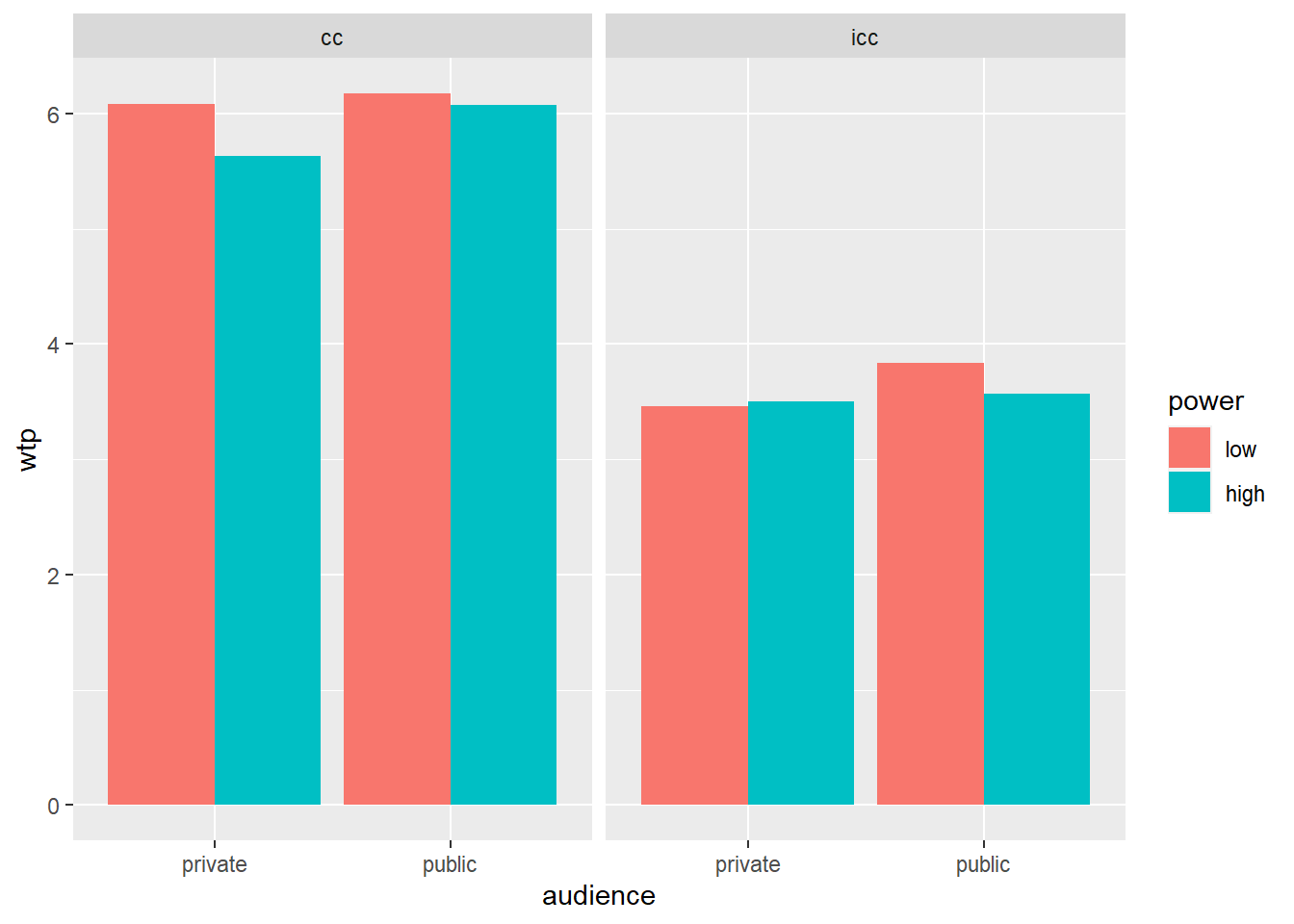
We can now formally test the three-way interaction:
# Specify the data, the dependent variable, the identifier (wid),
# the variable that represents the within-subjects condition, and the variables that represent the between subjects conditions.
ezANOVA(data = powercc.long, dv = wtp, wid = subject, within = consumption_type, between = power*audience)
## $ANOVA
## Effect DFn DFd F p p<.05 ges
## 2 power 1 139 1.867530e+00 1.739647e-01 9.061619e-03
## 3 audience 1 139 2.977018e+00 8.667716e-02 1.436772e-02
## 5 consumption_type 1 139 6.303234e+02 1.687352e-53 * 5.915501e-01
## 4 power:audience 1 139 5.801046e-03 9.393977e-01 2.840440e-05
## 6 power:consumption_type 1 139 4.719313e-01 4.932445e-01 1.083172e-03
## 7 audience:consumption_type 1 139 2.700684e-02 8.697041e-01 6.204919e-05
## 8 power:audience:consumption_type 1 139 2.982598e+00 8.638552e-02 6.806406e-03We see in these results that the three-way interaction between power, audience, and consumption type is marginally significant. You can report this as follows: “A repeated measures ANOVA established that the three-way interaction between power, audience, and consumption type, was marginally significant (F(1, 139) = 2.98, p = 0.086).