Chapter 3 Prediction and Inference
3.1 Prediction
Assume a GLM has been fitted, yielding \(\hat{\boldsymbol{\beta}}\in{\mathbb R}^{p}\). If we are given a new predictor vector \(\boldsymbol{x}_{0}\), we can compute \[\begin{equation} \hat{\eta}_{0} = \hat{\boldsymbol{\beta}}^{T}\boldsymbol{x}_{0} \end{equation}\]
Now, \[\begin{equation} {\mathrm{Var}}[\hat{\boldsymbol{\beta}}] \stackrel{a}{=} F^{-1}(\hat{\boldsymbol{\beta}}) \end{equation}\]
so \[\begin{equation} {\mathrm{Var}}[\hat{\eta}_{0}] \stackrel{a}{=} \boldsymbol{x}_{0}^{T}\;{\mathrm{Var}}[\hat{\boldsymbol{\beta}}] \;\boldsymbol{x}_{0} \stackrel{a}{=} \boldsymbol{x}_{0}^{T}\;F^{-1}(\hat{\boldsymbol{\beta}})\;\boldsymbol{x}_{0} \end{equation}\]
or, alternatively, \[\begin{equation} \text{SE}[\hat{\eta}_{0}] \stackrel{a}{=} \sqrt{x_{0}^{T}\;F^{-1}(\hat{\boldsymbol{\beta}})\;x_{0}} \end{equation}\]
A prediction for a new, unobserved \(y_{0}\) is then \[\begin{equation} \hat{y}_{0} = {\mathrm E}[Y |\hat{\boldsymbol{\beta}}, x_{0}] = h(\hat{\boldsymbol{\beta}}^{T}x_{0}) \end{equation}\]
An approximate \((1 - \alpha)\) confidence interval for \({\mathrm E}[Y |\boldsymbol{\beta}, x_{0}]\) is then \[\begin{equation} CI = \left[ h \left( \hat{\boldsymbol{\beta}}^{T} x_{0} - z_\frac{\alpha}{2} \sqrt{x_{0}^{T}\;F^{-1}(\hat{\boldsymbol{\beta}})\;x_{0}} \right) \;, \; h \left( \hat{\boldsymbol{\beta}}^{T} x_{0} + z_\frac{\alpha}{2} \sqrt{x_{0}^{T}\;F^{-1}(\hat{\boldsymbol{\beta}})\;x_{0}} \right) \right] \end{equation}\]
Note that this is not, in general, symmetric about \(h(\hat{\boldsymbol{\beta}}^{T}x_{0})\).
What about predictive intervals for \(y_{0}\), by analogy with the linear model case? These are more complicated, as they depend on the response distribution, and we do not consider them here.
3.1.1 Example: Hospital Stay Data
Predict the duration of stay for a new individual with age \(60\), and temperature \(99\).
We could try
##        1
## 2.595732
But this is not what we want - for GLMs, the predict function gives by default the value of the linear predictor.
To predict on the scale of the response, one needs
##       1
## 13.4064
or
##       1
## 13.4064
Similarly we aim to achieve a 95% confidence interval for the expected mean function at age 60 and temperature 99 as for the linear model as follows:
# Attempt, as for lm:
predict(hosp.glm, newdata=data.frame(age=60, temp1=99), type="response",
interval="confidence")
## 1
## 13.4064This does not work, so we need to do it manually!
# Compute the predicted linear predictor as above.
lphat  <- predict(hosp.glm, newdata=data.frame(age=60, temp1=99))

# Extract the covariance.
varhat <- summary(hosp.glm)$cov.scaled     # = F^(-1)(betahat)

# Define new data point
x0 = c(1, 60, 99)

# Compute the width of the interval for the linear predictor.
span   <- qnorm(0.975) * sqrt( x0 %*%  varhat %*%  x0)

# Compute the interval for the mean.
c(exp(lphat-span), exp(lphat+span))
## [1] 8.836973 20.3386013.2 Hypothesis Tests
We wish to test the values of \(\hat{\boldsymbol{\beta}}\), just as for linear models.
3.2.1 Simple Tests
We take as hypotheses \(\mathcal{H}_{0}: \boldsymbol{\beta} = \boldsymbol{b}\) and \(\mathcal{H}_{1}: \boldsymbol{\beta} \neq \boldsymbol{b}\).
3.2.1.1 Wald Test
An obvious candidate for a test statistic is the Mahalanobis distance of \(\hat{\boldsymbol{\beta}}\) from \(\boldsymbol{\beta}\), otherwise know as the Wald statistic. Under \(\mathcal{H}_{0}\), \[\begin{equation} W = (\hat{\boldsymbol{\beta}}- \boldsymbol{b})^{T}\;F(\hat{\boldsymbol{\beta}})\;(\hat{\boldsymbol{\beta}}- \boldsymbol{b}) \stackrel{a}{\sim} \chi^{2}(p) \end{equation}\]
The test is then:
- Reject \(\mathcal{H}_{0}\) at significance level \(\alpha\) if \(W > \chi^{2}_{p, \alpha}\).
3.2.1.2 Likelihood Ratio Test
An alternative is a likelihood ratio test. Define \[\begin{equation} \Lambda = 2\log \left( \frac{L(\hat{\boldsymbol{\beta}})}{L(\boldsymbol{\beta})} \right) = 2(\ell(\hat{\boldsymbol{\beta}}) - \ell(\boldsymbol{\beta})) \end{equation}\]
What is the distribution of \(\Lambda\)? Taylor-expanding \(\ell\), we find \[\begin{equation} \ell(\boldsymbol{\beta}) \stackrel{a}{=} \ell(\hat{\boldsymbol{\beta}}) + (\boldsymbol{\beta} - \hat{\boldsymbol{\beta}})^{T}S(\hat{\boldsymbol{\beta}}) - \frac{1}{2} (\boldsymbol{\beta} - \hat{\boldsymbol{\beta}})^{T}\;F(\hat{\boldsymbol{\beta}})\;(\boldsymbol{\beta} - \hat{\boldsymbol{\beta}}) \end{equation}\]
But \(S(\hat{\boldsymbol{\beta}}) = 0\), so we have \[\begin{equation} 2(\ell(\hat{\boldsymbol{\beta}}) - \ell(\boldsymbol{\beta})) \stackrel{a}{=} (\boldsymbol{\beta} - \hat{\boldsymbol{\beta}})^{T}\;F(\hat{\boldsymbol{\beta}})\;(\boldsymbol{\beta} - \hat{\boldsymbol{\beta}}) \stackrel{a}{\sim} \chi^{2}(p) \end{equation}\]
Under \(\mathcal{H}_{0}\), \(\boldsymbol{\beta} = \boldsymbol{b}\), so we have \[\begin{equation} \Lambda = 2(\ell(\hat{\boldsymbol{\beta}}) - \ell(\boldsymbol{b})) \stackrel{a}{\sim} \chi^{2}(p) \end{equation}\]
We then
- Reject \(\mathcal{H}_{0}\) at significance level \(\alpha\) if \(\Lambda > \chi^{2}_{p, \alpha}\).
3.2.2 Generalisation to Nested Models
Our hypotheses are now \[\begin{align} \mathcal{H}_{0}&: C\boldsymbol{\beta} = \gamma \\ \mathcal{H}_{1}&: C\boldsymbol{\beta} \neq \gamma \end{align}\]
where: \(C\in{\mathbb R}^{s\times p}\); \(\dim(\text{image}(C)) = s\); \(\gamma\in{\mathbb R}^{s}\).
The equation \(C\boldsymbol{\beta} = \gamma\) constrains the possible values of \(\boldsymbol{\beta}\), reducing the dimensionality of the space of possible solutions by \(s\). The set of \(\boldsymbol{\beta}\in{\mathbb R}^{p}\) satisfying \(C\boldsymbol{\beta} = \gamma\) forms a \((p - s)\)-dimensional affine subspace of \({\mathbb R}^{p}\). This therefore corresponds to a restricted or reduced model, as against \(\mathcal{H}_{1}\), which corresponds to the full model. We may sometimes say that \(\mathcal{H}_{0}\) is a submodel of \(\mathcal{H}_{1}\) because the parameter space of \(\mathcal{H}_{0}\) is a subset of the parameter space of \(\mathcal{H}_{1}\).
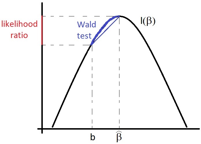
Figure 3.1: Illustration of the relationship between the Wald test and the likelihood ratio test.
3.2.2.1 Example
Let \[\begin{align} C & = \begin{pmatrix} 1 & 0 & 0 & \ldots & 0 \\ 0 & 1 & 0 & \ldots & 0 \end{pmatrix} \in {\mathbb R}^{2\times p} \\ \gamma & = 0 \in {\mathbb R}^{2} \end{align}\]
with \(\boldsymbol{\beta} \in{\mathbb R}^{p}\). Then \[\begin{equation} \mathcal{H}_{0}: \begin{cases} \beta_{1} = 0 & \\ \beta_{2} = 0 & \end{cases} \end{equation}\]
whereas \(\mathcal{H}_{1}\) has \(\beta_{1}\) and \(\beta_{2}\) unrestricted.
3.2.2.2 Wald Test
We have \[\begin{equation} W = (C\hat{\boldsymbol{\beta}} - \gamma)^{T}\; \left( C \;F^{-1}(\hat{\boldsymbol{\beta}})\;C^{T} \right)^{-1} \; (C\hat{\boldsymbol{\beta}} - \gamma) \stackrel{a}{\sim} \chi^{2}(s) \end{equation}\]
where, recall, \(s\) is the number of constraints; or, equivalently, the difference in the number of parameters; or, more abstractly, the difference in the dimensions of the parameter spaces.
3.2.2.3 Likelihood Ratio Test
We have \[\begin{equation} \Lambda = 2(\ell(\hat{\boldsymbol{\beta}}) - \ell(\tilde{\boldsymbol{\beta}})) \stackrel{a}{\sim} \chi^{2}(s) \end{equation}\]
where \(\hat{\boldsymbol{\beta}}\) is the MLE under \(\mathcal{H}_{1}\), while \(\tilde{\boldsymbol{\beta}}\) is the MLE under \(\mathcal{H}_{0}\), that is, the MLE for the restricted model.8
3.2.3 Example: Hospital Stay Data
Consider the hospital data. Construct a Gamma GLM with log link for the duration of hospital stay as a function of age and temp1, the temperature at admission, as follows
\[\begin{equation} \eta = \beta_{1} + \beta_{2}\texttt{age} + \beta_{3}\texttt{temp1} \end{equation}\]
where \[\begin{equation} \texttt{duration} |\texttt{age}, \texttt{temp1} \sim \text{Gamma}(\nu, \nu e^{-\eta}) \end{equation}\]
which can be coded in R as follows:
data(hosp, package="npmlreg")
hosp.glm <- glm(duration~age + temp1, data=hosp, family=Gamma(link=log))
Note that the parameterisation chosen means that, from properties of the Gamma distribution: \[\begin{align} \textrm{E}[\texttt{duration} |\texttt{age}, \texttt{temp1}] & = {\nu \over \nu e^{-\eta}} = e^{\eta} \\ \textrm{Var}[\texttt{duration} |\texttt{age}, \texttt{temp1}] & = {\nu \over (\nu e^{-\eta})^{2}} = {e^{2\eta} \over \nu} \end{align}\]
The first equation says that we are using a log link, i.e. an exponential response; the second equation identifies \(\phi = \tfrac{1}{\nu}\) and \(\mathcal{V}(\mu) = \mu^{2}\).
We now wish to test \[\begin{equation} \mathcal{H}_{0}: \beta_{3} = 0 \end{equation}\] against \[\begin{equation} \mathcal{H}_{1}: \beta_{3} \neq 0 \end{equation}\]
We note that \[\begin{equation} C = \begin{pmatrix} 0 & 0 & 1 \end{pmatrix} \in {\mathbb R}^{1 \times 3} \end{equation}\]
while \(\gamma = 0\), so that the constraint equation can be written \[\begin{equation} \begin{pmatrix} 0 & 0 & 1 \end{pmatrix} \begin{pmatrix} \beta_{1} \\ \beta_{2} \\ \beta_{3} \end{pmatrix} = 0 \end{equation}\]
The variance we are looking for is \[\begin{equation} C\;F^{-1}(\hat{\boldsymbol{\beta}})\;C^{T} = \begin{pmatrix} 0 & 0 & 1 \end{pmatrix} F^{-1}(\hat{\boldsymbol{\beta}}) \begin{pmatrix} 0 \\ 0 \\ 1 \end{pmatrix} = \text{Var}[\hat{\boldsymbol{\beta}}_{3}] = 0.028 \end{equation}\]
which can be obtained from R as follows:
##              (Intercept)           age         temp1
## (Intercept) 276.25822713 -3.728838e-02 -2.7943778049
## age          -0.03728838  3.246846e-05  0.0003656812
## temp1        -2.79437780  3.656812e-04  0.0282713219
The Wald statistic is then given by \[\begin{equation} W = {\hat{\boldsymbol{\beta}}_{3}^{2} \over \textrm{Var}[\hat{\boldsymbol{\beta}}_{3}]} = {(0.31)^{2} \over 0.028} = 3.32 \end{equation}\]
Since \(\chi^{2}_{1, 0.05} = 3.84\) and \(\chi^{2}_{1, 0.1} = 2.71\), we see that we do not reject \(\mathcal{H}_{0}\) at the \(5\%\) level, but do reject at the \(10\%\) level.
3.2.3.1 Does R give what one expects?
Notice that when \(\phi\) has to be estimated as well as \(\boldsymbol{\beta}\), we have a situation similar to an unknown variance in the testing of means, going under the title `small sample t-tests’.
For the example we are looking at, we have \[\begin{equation} \sqrt{W} = {\hat{\boldsymbol{\beta}}_{3} \over \text{SE}(\hat{\boldsymbol{\beta}}_{3})} = {0.31 \over 0.17} = 1.82 \end{equation}\]
This is the same as the number in the `\(t\)-value’ column in the R summary:
##
## Call:
## glm(formula = duration ~ age + temp1, family = Gamma(link = log),
##     data = hosp)
##
## Coefficients:
##               Estimate Std. Error t value Pr(>|t|)
## (Intercept) -28.654096  16.621018  -1.724   0.0987 .
## age           0.014900   0.005698   2.615   0.0158 *
## temp1         0.306624   0.168141   1.824   0.0818 .
## ---
## Signif. codes:  0 '***' 0.001 '**' 0.01 '*' 0.05 '.' 0.1 ' ' 1
##
## (Dispersion parameter for Gamma family taken to be 0.2690233)
##
##     Null deviance: 8.1722  on 24  degrees of freedom
## Residual deviance: 5.7849  on 22  degrees of freedom
## AIC: 142.73
##
## Number of Fisher Scoring iterations: 6
However, if \(W \sim \chi^{2}(1)\), then \(\sqrt{W} \sim {\mathcal N}(0, 1)\), leading to \[\begin{equation} p = 2(1 - \Phi(1.82)) = 0.068 \end{equation}\]
This number does not appear in the R summary. The explanation is that if \(\phi\) is estimated, R uses \(t_{n - p}\) rather than \({\mathcal N}(0, 1)\), leading to \[\begin{equation} p = 2(1 - \Phi_{t}(1.82)) = 0.082 \end{equation}\]
and this number does appear in the R summary.
The use of the \(t\) distribution rather than the Gaussian distribution accounts for the extra variability introduced by estimating \(\phi\). It still uses asymptotic normality as a foundation. In fact, R also allows one to assume the dispersion is known:
##
## Call:
## glm(formula = duration ~ age + temp1, family = Gamma(link = log),
##     data = hosp)
##
## Coefficients:
##               Estimate Std. Error z value Pr(>|z|)
## (Intercept) -28.654096  16.621017  -1.724  0.08471 .
## age           0.014900   0.005698   2.615  0.00892 **
## temp1         0.306624   0.168141   1.824  0.06821 .
## ---
## Signif. codes:  0 '***' 0.001 '**' 0.01 '*' 0.05 '.' 0.1 ' ' 1
##
## (Dispersion parameter for Gamma family taken to be 0.2690233)
##
##     Null deviance: 8.1722  on 24  degrees of freedom
## Residual deviance: 5.7849  on 22  degrees of freedom
## AIC: 142.73
##
## Number of Fisher Scoring iterations: 6
The resulting summary talks of a \(z\)-value rather than a \(t\)-value, and computes the corresponding \(p\) using a Gaussian distribution.
We will use \(\chi^{2}\) tests exclusively, thereby ignoring the variability introduced by the estimation of \(\phi\).
3.3 Confidence Regions for \(\hat{\boldsymbol{\beta}}\)
These follow from standard maximum likelihood theory. There are two popular types, which in general are not equivalent.
3.4 Issues with GLMs and the Wald Test
3.4.1 Separation
Consider a logistic regression problem with linear predictor: \(\eta = \beta_{1} + \beta_{2} x\). Suppose that the data has the following property (not so unreasonable): the \(x\) values of all the points with \(y = 0\) are less than the \(x\) values of all the points with \(y = 1\). This is illustrated in Figure 3.2.
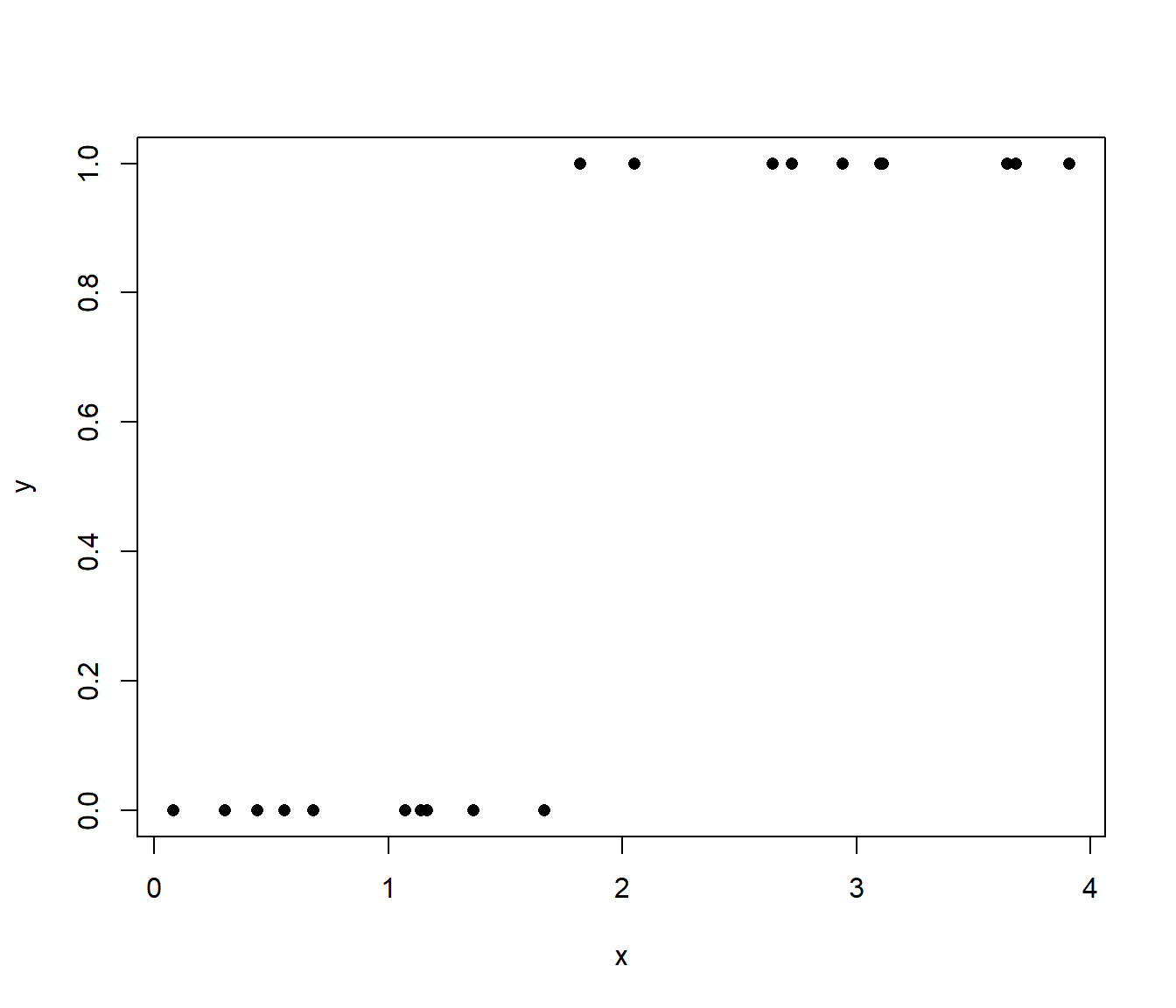
Figure 3.2: Illustration of `separated’ binary data.
Problem
What will be the estimated value \(\hat{\beta}_{2}\) of \(\beta_{2}\)? This question seems unanswerable, but in fact it has a very simple answer. First, consider reparameterising the linear predictor. Define \[\begin{align} \omega & = \beta_{2} \\ x_{0} & = - \frac{\beta_{1}}{\beta_{2}} \end{align}\]
The linear predictor is thus: \[\begin{equation} \eta = \omega (x - x_{0}) \end{equation}\]
The expression for the mean, that is, the probability that \(y = 1\) given \(x\), is then \[\begin{equation} \pi(x) = \frac{e^{\omega (x - x_{0})}}{1 + e^{\omega (x - x_{0})}} \end{equation}\]
The estimation task is to pick values of \(\omega\) and \(x_{0}\) that maximize the probability of the data. Clearly, if we can choose the parameters so that \(\pi(x) = 1\) for those points with \(y = 1\) and \(\pi(x) = 0\) for those points with \(y = 0\), we cannot do better: this is the maximum achievable with the model, equivalent to the saturated model in fact. Call this a perfect fit.
Now consider the following. Pick \(x_{0}\) so that it lies between the \(x\) with \(y = 0\) and the \(x\) with \(y = 1\). This must be possible because of the initial assumption about the data. Now note that for all the \(x\) with \(y = 0\), \((x - x_{0}) < 0\). If we let \(\omega\rightarrow\infty\), then \(\pi(x)\rightarrow 0\). On the other hand, for all the \(x\) with \(y = 1\), \((x - x_{0}) > 0\), so that as \(\omega\rightarrow\infty\), \(\pi(x)\rightarrow 1\). The limiting solution is thus a step function with the step at \(x_{0}\).
We can therefore achieve a perfect fit by allowing \(\omega\rightarrow\infty\). Unfortunately, this means that the linear predictor is not defined, and, practically speaking, the estimation algorithm will not converge.9
Of course, in this simple case, we can see what is happening, and can anticipate that a step function might be a solution. In general, however, this situation might be hard to detect, and hard to correct, at least within the framework of GLMs. So what is to be done?
Solution
Remember that we set out to model functional relationships. GLMs are one way to do this, by constraining the form of the function in a useful way. In this case, however, they seem to be too limiting. There are two reasons why this might be the case.
One is that the step function solution is appropriate for the data and context with which we are dealing. In this case, the main problem is that our set of functions is poorly parameterised, and includes the step function only as a singular limiting case. There is no real solution for this in the context of GLMs, although more general models could be used.
The other is that the step function solution is not appropriate, and that we really would expect a smoother solution. This is much harder to deal with in the context of classical statistics. We are saying that we expect the value of \(\omega\) to be finite, larger values becoming less and less probable, until in the limit, an infinite value is impossible. The only real way to deal with this situation is via a prior probability distribution on \(\omega\) or by imposing some regularising constraint, but those are another story and another course. Within the GLM world, one has simply to be aware of the possibility of separation, and that it may be caused by overly subdividing the data via categorical variables, that is, essentially by overfitting.
3.4.2 Hauck-Donner Effect
A related but independent effect was noted by Hauck and Donner (1976).
Consider \[\begin{equation} W = \frac{\hat{\boldsymbol{\beta}}^{2} }{{\mathrm{Var}}[\hat{\boldsymbol{\beta}}]} \end{equation}\]
If \(\hat{\boldsymbol{\beta}}\rightarrow\infty\) (e.g. in cases of separation), then it is quite likely that \({\mathrm{Var}}[\hat{\boldsymbol{\beta}}]\rightarrow\infty\) also. The result can be that the test statistic becomes very small, and in fact tends to zero! Hauck and Donner showed that:
- Wald’s statistic decreased to zero as the distance between the parameter estimate and the null value increased.
So, as one’s null hypothesis gets more and more wrong, the Wald statistic gets smaller and smaller, and one is decreasingly able to reject the increasingly wrong null.