Chapter 4 Deviance
4.1 Goodness-of-Fit
We would like to find a measure for goodness-of-fit, or, to put it another way, a measure for the discrepancy between the data \(\boldsymbol{y} \in \mathbb{R}^n\) and the fit \(\hat{\boldsymbol\mu} = (\hat{\mu}_1, \hat{\mu}_2, \ldots, \hat{\mu}_n) \in \mathbb{R}^n\), where \(\hat{\mu}_i = h(\boldsymbol\beta^T \boldsymbol{x}_i)\).
First we need to understand how well any GLM could be expected to fit.
4.1.1 The Saturated Model
The log likelihood at the MLE \(\hat{\boldsymbol{\beta}}\) is
\[ \ell(\hat{\boldsymbol\beta}) = \sum_i \left( \frac{y_i \hat{\theta}_i - b(\hat{\theta}_i)}{\phi_i} + c(y_i, \phi_i) \right). \tag{4.1} \]
The larger \(\ell(\hat{\boldsymbol\beta})\), the better the fit, but what is large? Consider the following. In the GLM, \(\boldsymbol\mu\), or equivalently \(\boldsymbol\theta = (\theta_1, \ldots, \theta_n)\), takes values in \(\mathbb{R}^n\). However, \(\mu_i = h(\boldsymbol\beta^T \boldsymbol{x}_i)\). Thus, as \(\boldsymbol\beta \in \mathbb{R}^n\) varies, \(\boldsymbol\mu = \{\mu_i\}\) can only trace out a \(p\)-dimensional submanifold of \(\mathbb{R}^n\): the possible values are constrained by the model structure. (Indeed, as we saw at the beginning, this is the whole point of the model in the first place.)
An upper bound for \(\ell(\hat{\boldsymbol{\beta}})\) would therefore be attained by a model that placed less constraints on \(\boldsymbol\mu\) (since maximisation over a superset necessarily produces a larger value). This can be achieved by simply allowing \(\boldsymbol\mu\) to range over all of \({\mathbb R}^{n}\), or in other words by allowing as many parameters as there are data points. This means intuitively that we end up `joining the dots’.
The maximum likelihood problem then breaks down into \(n\) simpler problems, as each term in equation (4.1) can be maximised separately. Differentiation with respect to \(\theta_{i}\) then gives \[\begin{equation} \ell_{i}'(\theta_{i}) = \frac{y_{i} - b'(\theta_{i})}{\phi_{i}} \end{equation}\]
leading to the MLE \(\hat{\boldsymbol\theta}\), or equivalently, \(\hat{\boldsymbol\mu}\), given by \[\begin{equation} y_{i} = b'(\hat{\theta}_{i}) = \hat{\mu}_{i} \end{equation}\]
This model, in which \(\boldsymbol\mu\) may vary over the whole of \({\mathbb R}^{n}\), and there is thus one parameter for each data point, is known as the saturated model. Its log likelihood at the MLE value \(\hat{\boldsymbol\mu}_{\text{sat}}\) is denoted \(\ell_{\text{sat}}\).
This then leads us to the notion of deviance.
4.1.2 Deviance
The deviance of a GLM is defined as follows: \[\begin{equation} D(\boldsymbol{Y}, \hat{\boldsymbol{\mu}}) = 2\;\phi\; \left( \ell_{\text{sat}} - \ell(\hat{\boldsymbol{\beta}}) \right) \end{equation}\]
while the scaled deviance is defined as \[\begin{equation} D_{\text{sc}}(\boldsymbol{Y}, \hat{\boldsymbol{\mu}}) = 2\; \left( \ell_{\text{sat}} - \ell(\hat{\boldsymbol{\beta}}) \right) \end{equation}\]
Now, \[\begin{equation} \ell(\hat{\boldsymbol{\beta}}) = \frac{1}{\phi} \sum_{i} m_{i}\; \left( y_{i}\hat\theta_{i} - b(\hat\theta_{i}) \right) + \sum_{i} c(y_{i}, \phi_{i}) \end{equation}\]
with \(\hat{\theta}_{i} = (b')^{-1}(\hat{\mu}_{i})\), and \(\phi_{i} = \frac{\phi}{m_{i}}\); and \[\begin{equation} \ell_{\text{sat}} = \frac{1}{\phi} \sum_{i} m_{i}\; \left( y_{i}\hat\theta_{\text{sat},i} - b(\hat{\theta}_{\text{sat},i}) \right) + \sum_{i} c(y_{i}, \phi_{i}) \end{equation}\]
with \(\hat{\theta}_{\text{sat},i} = (b')^{-1}(y_{i})\), that is, \(\hat{\mu}_{\text{sat},i} = y_{i}\). We thus have that \[\begin{equation} D(\boldsymbol{Y}, \hat{\boldsymbol{\mu}}) = 2 \sum_{i} m_{i} \left\{ y_{i} \left( \hat\theta_{\text{sat},i} - \hat\theta_{i} \right) - \left( b(\hat\theta_{\text{sat},i}) - b(\hat\theta_{i}) \right) \right\} \tag{4.2} \end{equation}\]
The deviance is thus independent of \(\phi\).
4.1.3 Example Special Cases
We now consider some examples. In these examples, we assume non-grouped data; that is, \(m_i=1\) and \(n=M\), where \(M\) is the number of groups. The results can easily be generalised to grouped data.
4.1.3.1 Gaussian
We have
- \(b(\theta_i) = \frac{1}{2}\theta_i^{2}\)
- \(\theta_i = (b')^{-1}(\mu_i) = \mu_i\)
We thus find that \[\begin{align} D(\boldsymbol{Y}, \hat{\boldsymbol{\mu}}) & = 2 \sum_{i} \left( y_{i}(y_{i} - \hat{\mu}_{i}) - \left( \frac{1}{2} y_{i}^{2} - \frac{1}{2} \hat{\mu}_{i}^{2} \right) \right) \\ & = 2 \sum_{i} \left( \frac{1}{2} y_{i}^{2} - y_{i}\hat{\mu}_{i} + \frac{1}{2} \hat{\mu}_{i}^{2} \right) \\ & = \sum_{i} (y_{i} - \hat{\mu}_{i})^{2} \end{align}\]
But this is just the residual sum of squares (RSS)!
4.1.3.2 Poisson
We have
- \(b(\theta_i) = e^{\theta_i}\)
- \(\theta_i = (b')^{-1}(\mu_i) = \log \mu_i\).
We thus find that \[\begin{align} D(\boldsymbol{Y}, \hat{\boldsymbol{\mu}}) & = 2 \sum_{i} \left( y_{i}(\log y_{i} - \log \hat{\mu}_{i}) - (y_{i} - \hat{\mu}_{i}) \right) \\ & = 2 \sum_{i} \left( y_{i} \log \left( \frac{y_{i}}{\hat{\mu}_{i}} \right) - (y_{i} - \hat{\mu}_{i}) \right) \end{align}\]
4.1.3.3 Bernoulli
We have
\(b(\theta_i) = \log(1 + e^{\theta_i})\)
\(\mu_i = \frac{e^{\theta_i}}{1 + e^{\theta_i}}\).
\(\theta_i = \log \frac{\mu_i}{1-\mu_i}\)
However, there is a problem. We have \[\begin{equation} \hat\theta_{\text{sat},i} = \log \left( \frac{y_{i}}{1 - y_{i}} \right) \end{equation}\]
for \(y_{i}\in\left\{0, 1\right\}\): the MLE \(\hat{\boldsymbol{\theta}}_{\text{sat}}\) is apparently not defined. However, this is easily solved. It is easiest to see if we write the maximum likelihood in terms of \(\hat{\boldsymbol{\mu}}\):
\[ \ell(\hat{\boldsymbol{\mu}}) = \sum_i \left( y_i \log\hat{\mu}_i + (1 - y_i) \log(1 - \hat{\mu}_i) \right). \]
The saturated log likelihood is therefore \[ \ell_{\text{sat}} = \sum_i \left( y_i \log y_i + (1 - y_i) \log(1 - y_i) \right) = 0 \]
for \(y_{i}\in \left\{0, 1\right\}\) by continuity.
We thus have
\[ \begin{aligned} D(\boldsymbol{Y}, \hat{\boldsymbol{\mu}}) &= -2 \, \ell(\hat{\boldsymbol\beta}) \\ &= -2 \sum_i \left( y_i \log\hat{\mu}_i + (1 - y_i)\log(1 - \hat{\mu}_i) \right) \\ &= -2 \left( \sum_{i : y_i = 0} \log(1 - \hat{\mu}_i) + \sum_{i : y_i = 1} \log\hat{\mu}_i \right). \end{aligned} \]
4.2 Asymptotic Properties
In order to use deviance effectively as a measure of goodness-of-fit, we need to be able to analyse its probabilistic behaviour, in order to perform tests, etc. Does deviance have, at least asymptotically, a nice distribution that we can use?
Looking at the form of the deviance, \[ \frac{D(\boldsymbol{Y}, \hat{\boldsymbol\mu})}{\phi} = 2 \; (\ell_{\text{sat}} - \ell(\hat{\boldsymbol\beta}) ), \]
one might suppose that, to be analogous with the quantities used in likelihood ratio tests, it would be \(\chi^2(n-p)\)-distributed asymptotically, since the saturated model has \(n\) parameters, and the model in which we are interested has \(p\). If this were the case, then we could say that if
\[ \frac{D(\boldsymbol{Y}, \hat{\boldsymbol\mu})}{\phi} > \chi^2_{p, \alpha} \tag{4.3} \]
then the model does not fit well.
Unfortunately, it is not true that \(\frac{D(\boldsymbol{Y}, \hat{\boldsymbol\mu})}{\phi}\) is asymptotically \(\chi^2\)-distributed in general. This is because the limit theorems that give the \(\chi^2\) distribution do not apply when the number of parameters varies as the amount of data increases. Here that is the case, as the dimensionality of the saturated model is not fixed, but \(n\).
In special cases, most notably for the Poisson distribution, or when the \(m_i \gg 1\), the asymptotics do hold, and we can use Equation (4.3) as a test of goodness-of-fit. In general, however, this is not the case.
Thus, as promising as deviance appears, it cannot serve as a complete replacement for the RSS, even though this is a special case. We will see, however, that deviance is still extremely useful.10
4.3 Pearson Statistic
We now take a slight detour to discuss an alternative measure of goodness-of-fit. This bears the same relationship to deviance that the Wald test bears to the likelihood ratio test: one works in the domain of the probability distribution; and one in its codomain, or in other words, in terms of probability itself.
The Pearson statistic is defined as \[ \chi^2_P = \sum_i m_i \frac{ (y_i - \hat{\mu}_i)^2 } { \mathcal{V}(\hat{\mu}_i) }. \]
We then see that \[ \begin{aligned} \frac{\chi^2_P}{\phi} &= \sum_i \frac{ (y_i - \hat{\mu}_i)^2 } { \frac{\phi}{m_i} \mathcal{V}(\hat{\mu}_i) } \\ &= \sum_i \frac{ (y_i - \hat{\mu}_i)^2 } { \widehat{\text{Var}}[y_i]} \\ &\stackrel{a}{\sim} \chi^2(n - p). \end{aligned} \]
Hence, \[ \chi^2_P \stackrel{a}{\sim} \phi \; \chi^2(n - p). \]
Thus \(\chi^2_P\) can be used to measure goodness-of-fit.
4.3.1 Relation to Deviance
Consider \(D(\boldsymbol{Y}, \hat{\boldsymbol\mu})\) for the Poisson model: \[ D(\boldsymbol{Y}, \hat{\boldsymbol\mu}) = 2 \sum_i \left( y_i \log \frac{y_i}{\hat{\mu}_i} - (y_i - \hat{\mu}_i) \right). \]
Expanding this as a function of \(\boldsymbol{y}\) around \(\hat{\boldsymbol\mu}\), we find \[ D(\boldsymbol{Y}, \hat{\boldsymbol\mu}) \simeq \sum_i \frac{(y_i - \hat{\mu}_i)^2}{\hat{\mu}_i}. \]
This is just the normal Pearson statistic for the Poisson distribution.
4.3.2 Pearson Residuals
We will see soon that we can define several types of residual for GLMs. One is defined based on the Pearson statistic, the `Pearson residual’: \[ r^P_i = \sqrt{m_i} \frac{y_i - \hat{\mu}_i}{\sqrt{\mathcal{V}(\hat{\mu}_i)}} = \sqrt{\hat{\phi}} \frac{y_i - \hat{\mu}_i}{ \sqrt{\widehat{\text{Var}}[y_i]}}. \]
If \(y_i \sim \mathcal{N}(\mu_i, \sigma^2)\), with \(m_i = 1\), then \(\mathcal{V}(\mu_i) = 1\), so that \[ r^P_i = y_i - \hat{\mu}_i = \epsilon_i. \]
Thus in a linear model, the Pearson residuals are just the `usual’ residuals.
4.3.3 Example: US Polio Data
This example concerns a Poisson model, so we can use deviance as a goodness-of-fit measure. We will use deviance and Pearson statistic to test if the model is a good fit.
The R code for this example is presented here:
# Load and plot the data
library("gamlss.data")
data("polio")
uspolio <- as.data.frame(matrix(c(1:168, t(polio)), ncol=2))
colnames(uspolio) <- c("time", "cases")

plot(uspolio, type="h")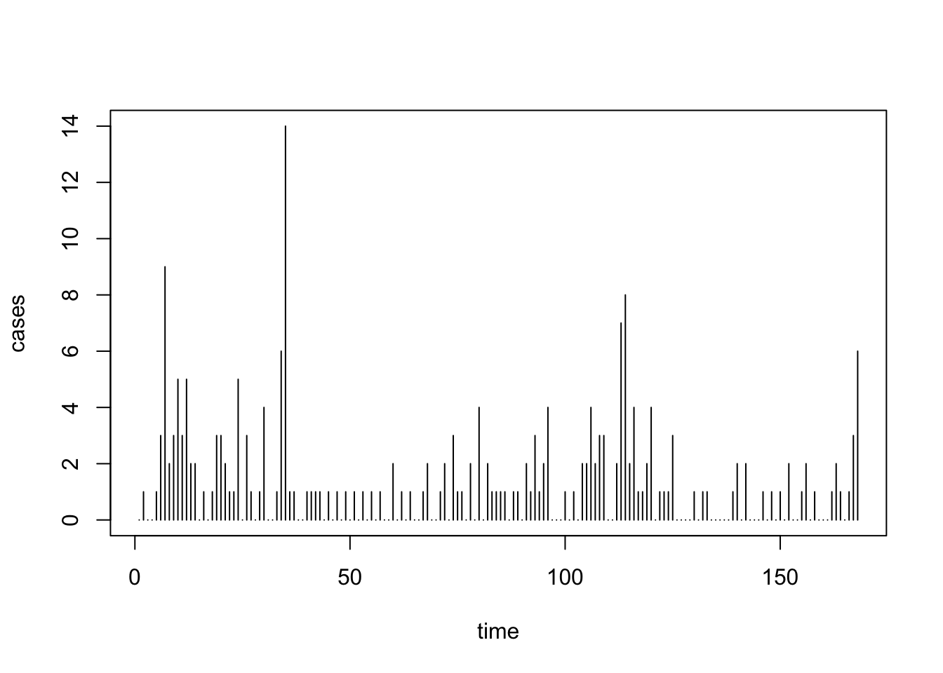
# Create Poisson GLM which includes time, six-month cycles
# and twelve-month cycles (see Estimation chapter)
polio2.glm<- glm(cases~time + I(cos(2*pi*time/12)) + I(sin(2*pi*time/12))
                 + I(cos(2*pi*time/6)) + I(sin(2*pi*time/6)),
                 family=poisson(link=log), data=uspolio)
summary(polio2.glm)
##
## Call:
## glm(formula = cases ~ time + I(cos(2 * pi * time/12)) + I(sin(2 *
## pi * time/12)) + I(cos(2 * pi * time/6)) + I(sin(2 * pi *
## time/6)), family = poisson(link = log), data = uspolio)
##
## Coefficients:
## Estimate Std. Error z value Pr(>|z|)
## (Intercept) 0.557241 0.127303 4.377 1.20e-05 ***
## time -0.004799 0.001403 -3.421 0.000625 ***
## I(cos(2 * pi * time/12)) 0.137132 0.089479 1.533 0.125384
## I(sin(2 * pi * time/12)) -0.534985 0.115476 -4.633 3.61e-06 ***
## I(cos(2 * pi * time/6)) 0.458797 0.101467 4.522 6.14e-06 ***
## I(sin(2 * pi * time/6)) -0.069627 0.098123 -0.710 0.477957
## ---
## Signif. codes: 0 '***' 0.001 '**' 0.01 '*' 0.05 '.' 0.1 ' ' 1
##
## (Dispersion parameter for poisson family taken to be 1)
##
## Null deviance: 343.00 on 167 degrees of freedom
## Residual deviance: 288.85 on 162 degrees of freedom
## AIC: 557.9
##
## Number of Fisher Scoring iterations: 5plot(1970 + ((uspolio$time-1)/12), uspolio$cases, type="h")
lines(1970 + ((uspolio$time-1)/12), polio2.glm$fitted,col=4)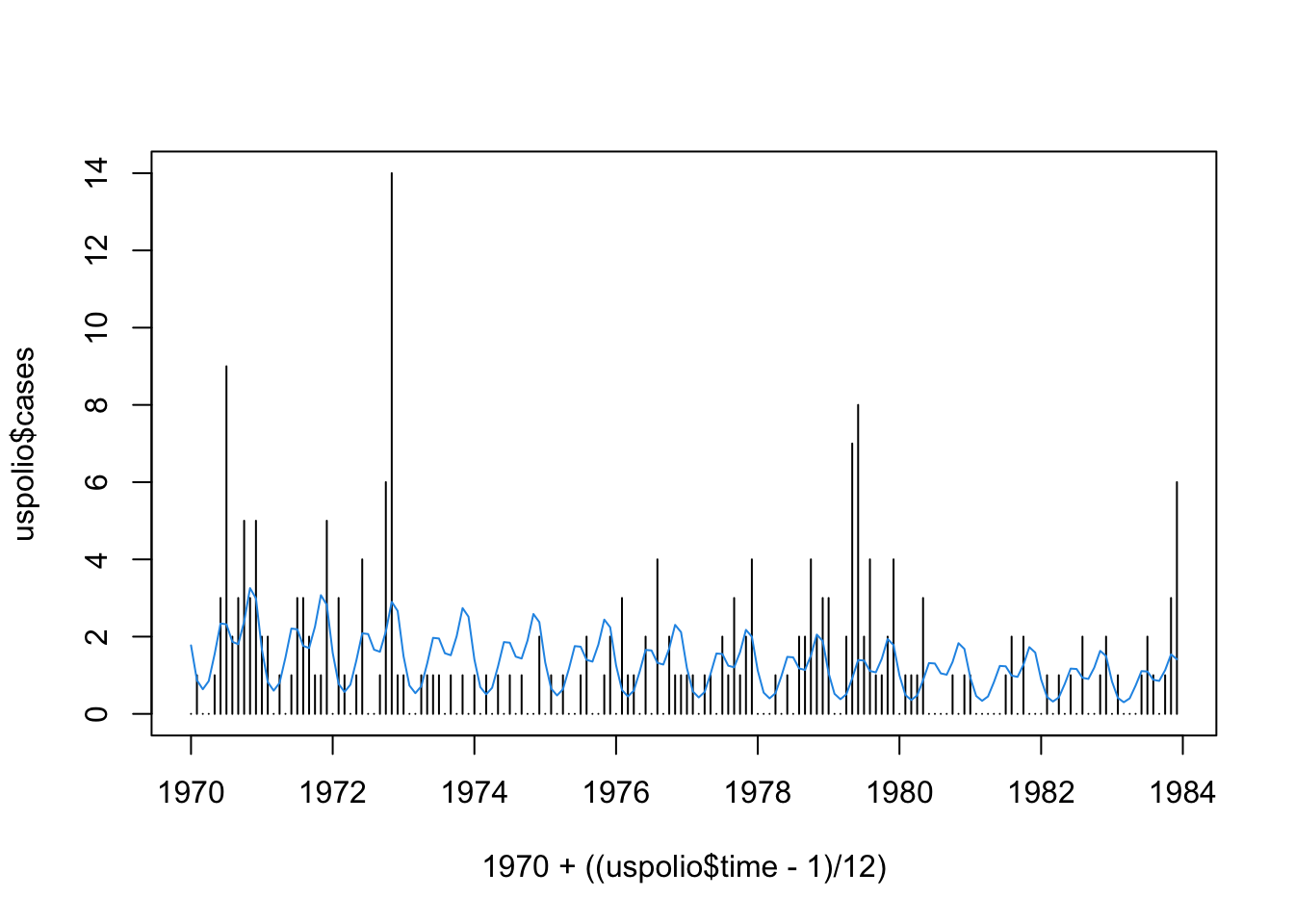
## [1] 288.8549## [1] 318.7216## [1] 192.7001The deviance is \(288.86\), while the Pearson statistic is \(318.72\). We have that \(\chi^2_{162, 0.05} = 192.7\), so either way we reject \(\mathcal{H}_0\), which is that the model is adequate, at \(5\%\). (The test is of a model with \(6\) parameters against a model with \(168\) parameters, hence the \(\chi^2\) distribution has \(162\) degrees of freedom.)
We can also test the model with temperature data.
# Read in temperature data and scale it
temp_data <- rep(c(5.195, 5.138, 5.316, 5.242, 5.094, 5.108, 5.260, 5.153,
                   5.155, 5.231, 5.234, 5.142, 5.173, 5.167), each = 12 )
scaled_temp = 10 * (temp_data - min(temp_data))/(max(temp_data) - min(temp_data))
uspolio$temp = scaled_temp

# Construct GLM
polio3.glm <- glm(cases~time + temp
                  + I(cos(2*pi*time/12)) + I(sin(2*pi*time/12))
                  + I(cos(2*pi*time/6)) + I(sin(2*pi*time/6)),
                  family=poisson(link=log), data=uspolio)
summary(polio3.glm)
##
## Call:
## glm(formula = cases ~ time + temp + I(cos(2 * pi * time/12)) +
## I(sin(2 * pi * time/12)) + I(cos(2 * pi * time/6)) + I(sin(2 *
## pi * time/6)), family = poisson(link = log), data = uspolio)
##
## Coefficients:
## Estimate Std. Error z value Pr(>|z|)
## (Intercept) 0.129643 0.186352 0.696 0.486623
## time -0.003972 0.001439 -2.761 0.005770 **
## temp 0.080308 0.023139 3.471 0.000519 ***
## I(cos(2 * pi * time/12)) 0.136094 0.089489 1.521 0.128314
## I(sin(2 * pi * time/12)) -0.531668 0.115466 -4.605 4.13e-06 ***
## I(cos(2 * pi * time/6)) 0.457487 0.101435 4.510 6.48e-06 ***
## I(sin(2 * pi * time/6)) -0.068345 0.098149 -0.696 0.486218
## ---
## Signif. codes: 0 '***' 0.001 '**' 0.01 '*' 0.05 '.' 0.1 ' ' 1
##
## (Dispersion parameter for poisson family taken to be 1)
##
## Null deviance: 343.00 on 167 degrees of freedom
## Residual deviance: 276.84 on 161 degrees of freedom
## AIC: 547.88
##
## Number of Fisher Scoring iterations: 5plot(1970 + ((uspolio$time-1)/12), uspolio$cases, type="h")
lines(1970 + ((uspolio$time-1)/12), polio3.glm$fitted, col="red")
## [1] 276.8357## [1] 279.2618## [1] 191.6084Note here that the \(\chi^2\) distribution has \(161\) degrees of freedom. From the results, we still reject \(\mathcal{H}_{0}\), although the deviance and Pearson statistic both reduced.
4.4 Residuals and Diagnostics
Just as there were two types of hypothesis test, and two measures of goodness-of-fit, there are two types of residual typically used for GLMs. These are as follows:
\[\begin{align*} \textrm{Deviance residuals} & \qquad & \textrm{Pearson residuals} \\ D = \sum_i d_i & \qquad & \chi^2_P = \sum_i m_i\frac{(y_i - \hat{\mu}_i)^2}{\mathcal{V}(\hat{\mu}_i)} \\ r^D_i = \textrm{sign}(y_i - \hat{\mu}_i)\sqrt{d_i} & & r^P_i = \sqrt{m_i}\frac{y_i - \hat{\mu}_i} { \sqrt{\mathcal{V}(\hat{\mu}_i)}} \end{align*}\]
Here \(d_i\) is the contribution of point (or data group) \(i\) to the overall deviance. That is, \[ d_i = 2 \, m_i \, \left\{ y_i \left( \hat{\theta}_{\text{sat}, i} - \hat{\theta}_i \right) - \left( b(\hat{\theta}_{\text{sat}, i}) - b(\hat{\theta}_i) \right) \right\} \] in Equation (4.2).
Just as in a linear model, the \(r^D_i\) or \(r^P_i\) can be plotted against \(i\) or against individual predictors, to detect violations of model assumptions. There is a problem though: neither \(r^D_i\) nor \(r^P_i\) is Gaussian. This makes `knowing what to look for’ in such plots somewhat tricky.
As a result, many modifications and transformations have been suggested: ‘adjusted deviance residuals’, ‘Anscombe residuals’, etc. We will not study these, but content ourselves with checking plots for suspicious looking patterns.
4.4.1 Example: Hospital Stay Data
data(hosp, package="npmlreg")
hosp.glm <- glm(duration~age+temp1, data=hosp, family=Gamma(link=log))

par(mfrow=c(2,2))
plot(residuals(hosp.glm, type="deviance"))
plot(hosp.glm$fitted, residuals(hosp.glm, type="pearson"))
plot(hosp$age, residuals(hosp.glm, type="deviance"))
plot(hosp$temp1, residuals(hosp.glm, type="deviance"))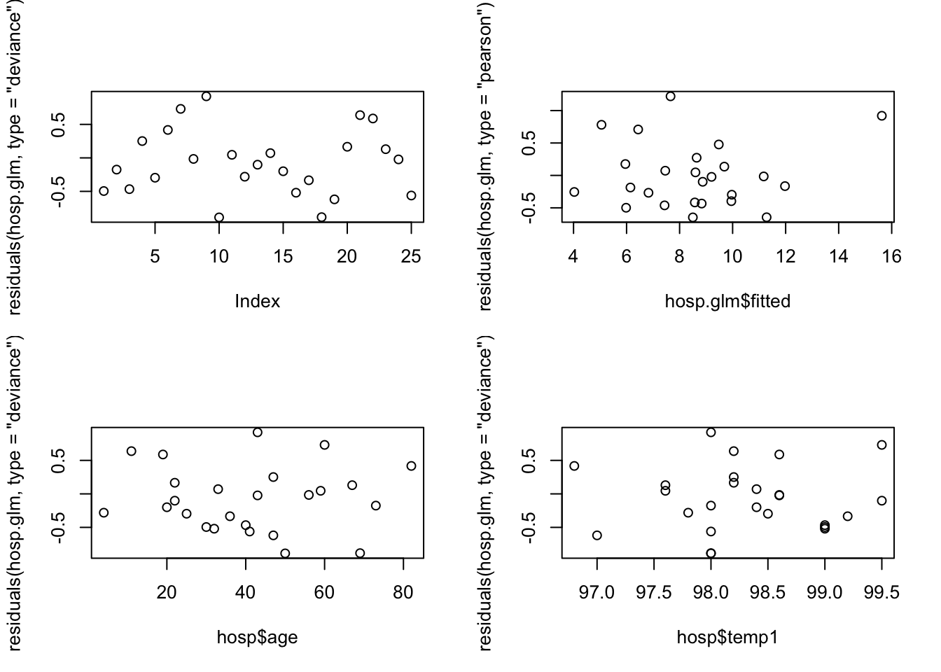
There are no obvious patterns here, but the sample size is quite small, which makes it more difficult. We can also compute and check autocorrelations.
## [1] 0.1430499## [1] 0.1444896Note that there are still some positive autocorrelations here, but again, the sample size is quite small for an accurate interpretation.
4.4.2 Example: US Polio Data
# For polio2 model
par(mfrow=c(2,1))
plot(uspolio$time, uspolio$cases, type="h")
lines(uspolio$time, polio2.glm$fitted, col="blue")
plot(uspolio$time, residuals(polio2.glm, type="deviance"), type="b")
abline(a=0,b=0)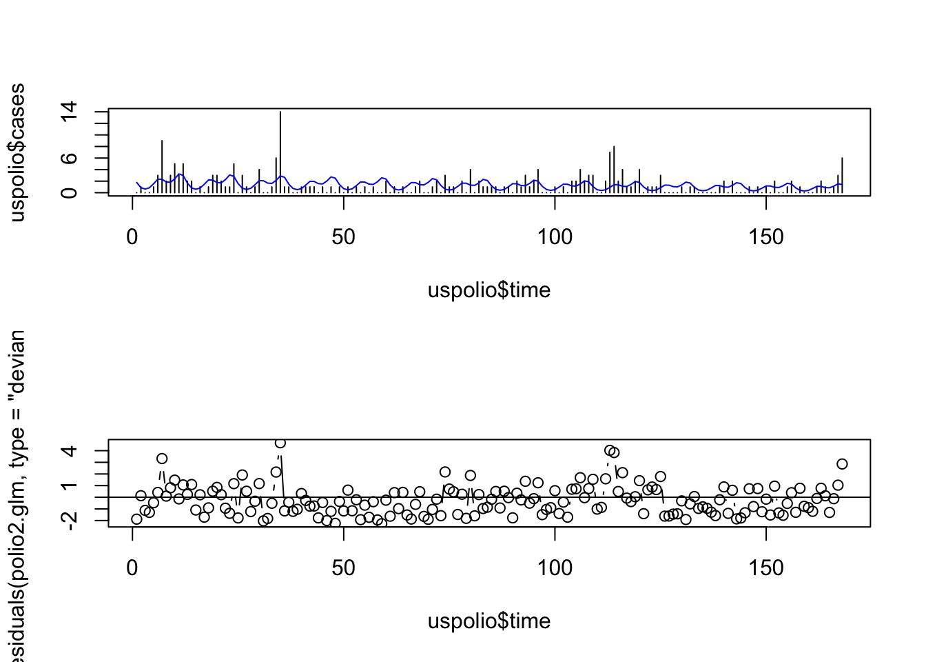
# For polio3 model
par(mfrow=c(2,1))
plot(uspolio$time, uspolio$cases, type="h")
lines(uspolio$time, polio3.glm$fitted, col="red")
plot(uspolio$time, residuals(polio3.glm, type="deviance"), type="b")
abline(a=0,b=0)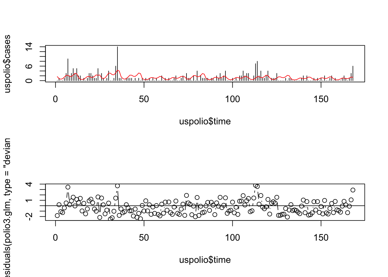
Here there is clearly residual autocorrelation present, so that the independence of different \(y_i\) is violated. We also compute the autocorrelations.
## [1] 0.1677067## [1] 0.1235241Note that the autocorrelation reduced in the second model but is still high.
4.5 Analysis of Deviance
The analysis of deviance is based on comparing the deviance of a model, not with the `perfect’ saturated model (which in practice is not perfect, since it overfits), but with the deviance of other competing models. These differences of deviances are much more useful in practice than the deviance itself.
Consider two nested GLMs \(\tilde{\mathcal{M}}\subset \mathcal{M}\).11 For example, \(\tilde{\mathcal{M}}\) could be the null model with \(g(\mu) = \beta_{1}\) and \(\mathcal{M}\) could be our model with \(g(\mu) = \boldsymbol{\beta}^{T}\boldsymbol{x}\), where \(\boldsymbol{\beta}\in{\mathbb R}^{p}\). More generally:
Let \(\mathcal{M}\) be a GLM, the `full’ model;
Let \(\tilde{\mathcal{M}}\) be a GLM nested in \(\mathcal{M}\), the `reduced’ model, with \[\begin{equation} C\boldsymbol{\beta} = \gamma \end{equation}\] with \(C \in {\mathbb R}^{s\times p}\).
Let \(\hat{\boldsymbol{\beta}}\) be the MLE under \(\mathcal{M}\);
Let \(\tilde{\boldsymbol{\beta}}\) be the MLE under \(\tilde{\mathcal{M}}\).
Then we define \[\begin{align} D(\tilde{\mathcal{M}}, \mathcal{M}) & = D(\tilde{\mathcal{M}}) - D(\mathcal{M}) \\ & = 2\;\phi\; \big( \ell_{\text{sat}} - \ell(\tilde{\boldsymbol{\beta}}) \bigr) - 2\;\phi\; \bigl( \ell_{\text{sat}} - \ell(\hat{\boldsymbol{\beta}}) \bigr) \\ & = 2\;\phi\; \bigl( \ell(\hat{\boldsymbol{\beta}}) - \ell(\tilde{\boldsymbol{\beta}}) \bigr) \end{align}\]
Note that \[\begin{equation} \frac{1 }{ \phi} D(\tilde{\mathcal{M}}, \mathcal{M}) = 2\bigl(\ell(\hat{\boldsymbol{\beta}}) - \ell(\tilde{\boldsymbol{\beta}})\bigr) \end{equation}\]
This is just the likelihood ratio statistics, and thus \[\begin{equation} \frac{1 }{ \phi} D(\tilde{\mathcal{M}}, \mathcal{M}) \stackrel{a}{\sim} \chi^{2}(s) \end{equation}\] where \(s\) is the number of constraints, that is, the difference in the dimensions of the parameter spaces, or the difference in the number of parameters.
From the definition of \(D(\tilde{\mathcal{M}}, \mathcal{M})\), we have that \[\begin{equation} D(\tilde{\mathcal{M}}) = D(\tilde{\mathcal{M}}, \mathcal{M}) + D(\mathcal{M}) \end{equation}\]
In words, “the discrepancy between the data and \(\tilde{\mathcal{M}}\) is equal to the discrepancy between the data and \(\mathcal{M}\) plus the discrepancy between \(\mathcal{M}\) and \(\tilde{\mathcal{M}}\).”
4.5.1 Interpretation and Testing
Consider applying this idea in the linear model case. There we have the following: \[\begin{equation} \sum_{i}(y_{i} - \tilde{\boldsymbol{\beta}}^{T}\boldsymbol{x}_i)^{2} = D(\tilde{\mathcal{M}}, \mathcal{M}) + \sum_{i}(y_{i} - \hat{\boldsymbol{\beta}}^{T}\boldsymbol{x}_i)^{2} \end{equation}\]
The left-hand side is the RSS of the reduced model, while the second term on the right-hand side is the RSS of the full model.
In this context, we know we have the partial \(F\)-test, based on the statistic: \[\begin{equation} F = \frac{ \bigl( \text{RSS reduced} - \text{RSS full} \bigr) / s }{ \bigl( \text{RSS full} / (n - p) \bigr)} \sim F(s, n - p) \end{equation}\]
We then apply this as follows: if \(F > F_{s, n - p, \alpha}\), we reject \(\mathcal{H}_{0}: \tilde{\mathcal{M}}\) in favour of \(\mathcal{H}_{1}: \mathcal{M}\) at level \(\alpha\).
How should we adapt this to the GLM case? By strict analogy, we have \[\begin{equation} F = \frac{D(\tilde{\mathcal{M}}, \mathcal{M}) / s }{ \hat\phi} = \frac{1}{s} \frac{D(\tilde{\mathcal{M}}, \mathcal{M}) }{ \hat\phi} \sim \frac{1}{s} \chi^{2}(s) \end{equation}\] where the latter, distributional result is true if we know \(\phi\), or if we simply ignore the extra variability introduced by estimating it.
In practice, we compute \(s F = \frac{D(\tilde{\mathcal{M}}, \mathcal{M})}{\hat\phi}\) and reject \(\mathcal{H}_{0}: \tilde{\mathcal{M}}\) if \(\frac{D(\tilde{\mathcal{M}}, \mathcal{M})}{\hat\phi} > \chi^{2}_{s, \alpha}\).
4.5.2 General Case
More generally we may have a series of nest models: \(\mathcal{M}_{1}\subset \mathcal{M}_{2}\subset \dotsb \subset \mathcal{M}_{N}\), that is, \(\mathcal{M}_{i}\subset \mathcal{M}_{i + 1}\) for \(i\in [1.. (N - 1)]\). We can then write down the following telescoping sum: \[\begin{align} D(\mathcal{M}_{1}) & = \sum_{i = 1}^{N - 1} D(\mathcal{M}_{i}, \mathcal{M}_{i + 1}) + D(\mathcal{M}_{N}) \\ & = \sum_{i = 1}^{N - 1} \bigl( D(\mathcal{M}_{i}) - D(\mathcal{M}_{i + 1}) \bigr) + D(\mathcal{M}_{N}) \\ & = \sum_{i = 1}^{N - 1} D(\mathcal{M}_{i}) - \sum_{i = 2}^{N} D(\mathcal{M}_{i}) + D(\mathcal{M}_{N}) \\ & = D(\mathcal{M}_{1}) - D(\mathcal{M}_{N}) + D(\mathcal{M}_{N}) \\ & = D(\mathcal{M}_{1}) \end{align}\]
A tabular representation of this sum is produced in R when the anova command is applies to a fitted GLM, as the next example demonstrates.
4.5.3 Example: Hospital Stay Data
Here analysis of deviance is applied to the full model for the hospital data, with the linear predictor: \[\begin{equation} \eta = \beta_{1} + \beta_{2}\texttt{age} + \beta_{3}\texttt{temp1} + \beta_{4}\texttt{wbc1} + \beta_{5}\texttt{antib} + \beta_{6}\texttt{bact} + \beta_{7}\texttt{serv}, \end{equation}\] Gamma family, and log link, as shown below:
data(hosp, package="npmlreg")

# Full model
fit1<- glm(duration~age+temp1+wbc1+antib+bact+serv, data=hosp,
           family=Gamma(link=log))

summary(fit1)
##
## Call:
## glm(formula = duration ~ age + temp1 + wbc1 + antib + bact +
## serv, family = Gamma(link = log), data = hosp)
##
## Coefficients:
## Estimate Std. Error t value Pr(>|t|)
## (Intercept) -18.925401 17.540130 -1.079 0.295
## age 0.010026 0.006636 1.511 0.148
## temp1 0.219006 0.178154 1.229 0.235
## wbc1 0.001654 0.044930 0.037 0.971
## antib -0.346060 0.242145 -1.429 0.170
## bact 0.075859 0.280639 0.270 0.790
## serv -0.291875 0.255843 -1.141 0.269
##
## (Dispersion parameter for Gamma family taken to be 0.2661922)
##
## Null deviance: 8.1722 on 24 degrees of freedom
## Residual deviance: 5.1200 on 18 degrees of freedom
## AIC: 147.57
##
## Number of Fisher Scoring iterations: 10## [1] 0.2661922## Analysis of Deviance Table
##
## Model: Gamma, link: log
##
## Response: duration
##
## Terms added sequentially (first to last)
##
##
## Df Deviance Resid. Df Resid. Dev
## NULL 24 8.1722
## age 1 1.38428 23 6.7879
## temp1 1 1.00299 22 5.7849
## wbc1 1 0.03236 21 5.7526
## antib 1 0.31246 20 5.4401
## bact 1 0.00017 19 5.4400
## serv 1 0.31995 18 5.1200The resulting anova table has the significance shown in the table in Figure 4.1.
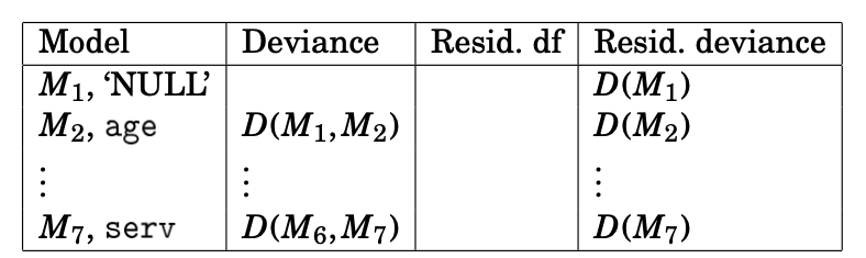
Figure 4.1: R output from an anova command on a GLM.
Each row represents the model containing the predictors in that row and all the previous rows.
From the definition of \(D(\tilde{\mathcal{M}}, \mathcal{M})\), in each row, the sum of the \(\texttt{Resid. deviance}\) and the \(\texttt{Deviance}\) gives the \(\texttt{Resid. deviance}\) in the row above.
If the
anovacommand is run with the argumenttest = "Chisq", then there will be an extra column in the table (see the code below). This represents the \(p\) value of a \(\chi^{2}\) test applied to the \(\texttt{deviance}\) in that row. It therefore tests the model in row above against the model in the row in which it appears.
## Analysis of Deviance Table
##
## Model: Gamma, link: log
##
## Response: duration
##
## Terms added sequentially (first to last)
##
##
##       Df Deviance Resid. Df Resid. Dev Pr(>Chi)
## NULL                     24     8.1722
## age    1  1.38428        23     6.7879  0.02258 *
## temp1  1  1.00299        22     5.7849  0.05224 .
## wbc1   1  0.03236        21     5.7526  0.72735
## antib  1  0.31246        20     5.4401  0.27862
## bact   1  0.00017        19     5.4400  0.97990
## serv   1  0.31995        18     5.1200  0.27293
## ---
## Signif. codes:  0 '***' 0.001 '**' 0.01 '*' 0.05 '.' 0.1 ' ' 1
We can use the results in the deviance table to perform different tests. Below are some examples.
4.5.3.1 Test Problem 1
Test \(\mathcal{H}_0: \mathcal{M}_1\), the null model where \(g(\eta) = \beta_1\), against \(\mathcal{H}_1: \mathcal{M}_7\), the full model. This is the analogue of a full \(F\) test.
From the table we read that \(D(\mathcal{M}_1) = 8.17\) while \(D(\mathcal{M}_7) = 5.12\). We also see from the R output that \(\hat{\phi} = 0.27\). We therefore have \[ \frac{D(\mathcal{M}_1, \mathcal{M}_7)}{\hat{\phi}} = \frac{8.17 - 5.12}{ 0.27} = \frac{3.05}{0.27} = 11.47. \]
This quantity is approximately \(\chi^2(6)\) distributed as \(\mathcal{M}_7\) has \(6\) more parameters than \(\mathcal{M}_1\). We find the \(p\) value using \(\texttt{R}\): \[ p = 1 - \texttt{pchisq}(11.47, 6) = 0.075. \]
We would thus just reject \(\mathcal{H}_0\) at the \(7.5\%\) level, quite weak evidence that the model explains anything at all.
Note the intuition here. If \(D(\tilde{\mathcal{M}}, \mathcal{M})\) is large, it means that the more complex model \(\mathcal{M}\) is doing a much better job at explaining the data than the simpler model \(\tilde{\mathcal{M}}\). If it is enough better, then we will reject \(\mathcal{H}_{0}: \tilde{\mathcal{M}}\). At the same time, when \(D(\tilde{\mathcal{M}}, \mathcal{M})\) is large, it means that the \(\chi^{2}\) value will be large and thus that the \(p\) value will be small, meaning that there is a small probability of finding our value of \(D(\tilde{\mathcal{M}}, \mathcal{M})\) or greater, if \(\mathcal{H}_{0}\) is true and \(\tilde{\mathcal{M}}\) is the correct model. Thus the smaller the \(p\) value, the less favourably we look on the null hypothesis and the more significant the level at which we can reject (more significance but smaller level number: we need \(p < 0.05\) to reject at \(5\%\), but \(p < 0.01\) to reject at \(1\%\)).
4.5.3.2 Test Problem 2
Now we take \(\mathcal{H}_0: \mathcal{M}_2\), with \(\eta = \beta_1 + \beta_2\texttt{age}\), and \(\mathcal{H}_1: \mathcal{M}_3\), with \(\eta = \beta_1 + \beta_2\texttt{age} + \beta_3\texttt{temp1}\). These correspond to successive levels in the table, and so we can read the deviance directly from the table. We then find \[ \frac{D(\mathcal{M}_2, \mathcal{M}_3)}{\hat{\phi}} = \frac{1.003}{0.27} = 3.77. \]
This quantity is (approximately) \(\chi^2(1)\) distributed, as there is one parameter difference between the two models. The \(p\) value is \[ p = 1 - \texttt{pchisq}(3.77, 1) = 0.052. \]
Thus, given \(\texttt{age}\), there is some weak evidence to support adding \(\texttt{temp1}\) to the model: we can reject \(\mathcal{H}_0\) at the \(5.2\%\) level.
4.5.3.3 Test Problem 3
Now we take \(\mathcal{H}_0: \mathcal{M}_3\), with \(\eta = \beta_1 + \beta_2\texttt{age} + \beta_3\texttt{temp1}\), and \(\mathcal{H}_1: \mathcal{M}_7\). Reading from the table, we find \(D(\mathcal{M}_7) = 5.12\), while \(D(\mathcal{M}_3) = 5.79\). This gives \[ \frac{D(\mathcal{M}_3, \mathcal{M}_7)}{\hat{\phi}} = \frac{5.79 - 5.12}{ 0.27} = 2.50. \]
This quantity is (approximately) \(\chi^2(4)\) distributed. The \(p\) value is \[ p = 1 - \texttt{pchisq}(2.50, 4) = 0.65. \]
There is thus no evidence at all for including any variable beyond \(\texttt{age}\) and \(\texttt{temp1}\).
One could argue that it is a good thing that deviance cannot be used as a general measure of goodness-of-fit, as it forces one to consider comparing one model against another. The idea that there is a measure of goodness-of-fit that applies in the absence of an alternative model is quite a dubious one.↩︎
Model \(\tilde{\mathcal{M}}\) is `nested’ in model \(\mathcal{M}\) when the parameter space of \(\tilde{\mathcal{M}}\) is a subset of the parameter space of \(\mathcal{M}\).↩︎