4 R Markdown

R Markdown provides an easy way to produce a rich, fully-documented reproducible analysis. It allows its user to share a single file that contains all of the commentary, R code, and metadata needed to reproduce the analysis from beginning to end. R Markdown allows for chunks of R code to be included along with Markdown text to produce a nicely formatted HTML, PDF, or Word file without having to know any HTML or LaTeX code or have to fuss with getting the formatting just right in a Microsoft Word DOCX file.

One R Markdown file can generate a variety of different formats and all of this is done in a single text file with a few bits of formatting. I think you’ll be pleasantly surprised at how easy it is to write an R Markdown document after your first few encounters.

4.1 Fixing Errors in an R Markdown file

We now shift back to the R Markdown file called first_rmarkdown.Rmd created in Chapter 3. We know that we left some errors in the creation of variables there, and while it might seem strange to show you errors, it is good exposure for someone new to this to see what errors one might see initially. We are going to see what happens when we click the Knit HTML button with these errors. Then we will clean up the code and see what the resulting file looks like from the Knit.

Figure 4.1: Errors in an R Markdown file

When you initially created an R Markdown file, a basic template with some code and text was inputted for you. This is to give you a sense of how to create your own R Markdown file with your own R code and your own commentary. We modified some of that code here. I decided to remove all of the lines in the cars named chunk of code even though the errors did not occur in the declaration of the objects that had names stored in them. We see that an HTML file is produced in the Viewer pane because View in Pane was selected.

As you look over the Including Plots text you may be surprised to see that there is no plot provided in the R Markdown file, but in the HTML file there is a scatter-plot showing temperature and pressure varying. This is something alluded to earlier. R Markdown runs the code stored in R chunks and then places that output into the HTML (or PDF or DOCX, etc.) format.

You can also see that the text appears as commentary before and after the R code. You’ll understand in a bit why the text “Including Plots” is so much larger than the other text.

Important note: Remember that all of the R code you want to run needs to be stored in a chunk (in the right order) for your analysis to be reproducible AND for you not to receive errors when you Knit. It is easy to do a lot of work in the R Console and then forget to add that work into a chunk in your Rmd file. This is probably the number one error you will see when you first begin working in RStudio. An example of this error is below in a GIF file.

Figure 4.2: Forgetting to copy from Console to R chunk

The object not found errors are the most frequently encountered errors and along with misspellings and not completing R code segments provide the vast majority of issues with R. You’ll see a further breakdown of this in Chapter 6.

4.2 The Components of an R Markdown File

4.2.1 YAML

The top part of the file is called the YAML header. YAML stands for “YAML Ain’t Markup Language” and its website at http://yaml.org makes the following statement as to what it is:

YAML is a human friendly data serialization standard for all programming languages.

Essentially, the YAML stores the metadata needed for the document. You can see an example of a YAML header from our first_rmarkdown.Rmd file:

---
title: "First RMarkdown"
author: "Chester Ismay"
output: html_document
---

There are many other fields that can be customized in the YAML header. The important thing to notice here are the three hyphens that begin and end the YAML header. Indentation also plays a role with YAML so be careful with your alignment of text.

4.2.2 Headers

Figure 4.3: Headers start with hashtags

As you can see above, you can create a lot of different sized headers by simply adding one or more # in front of the text you’d like to denote the header.

4.2.3 Emphasis

Whenever you see a hash-tag in the text of your R Markdown document, you now know that this will correspond to bolded larger text² that denotes the start of a section of your document.

This is one of the nice features of R Markdown. You can simply look at the plain text and know what it will produce in the knitted document. We can also add different styles of emphasis to words, phrases, or sentences by surrounding them in matching symbols. Below are some examples.

Figure 4.4: Different emphasis styles in Markdown

You are beginning to see how easy it is to customize your output. We’ll next discuss ways to add links to URLs, create ordered and unordered lists, and other frequently used Markdown features.

4.2.4 Links

To add a link to a URL, you simply enclose the text you’d like displayed in the resulting HTML file inside [ ] and then the link itself inside ( ) right next to each other with no space in between.

Figure 4.5: Links to webpages

4.2.5 Lists

The GIF below shows the process of creating both ordered and unordered lists.

Figure 4.6: Ordered and unordered lists

Note that only numbers are needed as we saw by numbering “Warm up food” with a “1.” We can also combine unordered and ordered lists by indenting the text two spaces.

In many of the examples that follow, you will see the actual text you’d type into your R Markdown document highlighted with a gray background and also the results of that text immediately below it.

1. Wake up
  - Get out of bed
1. Warm up food
  - Open kitchen door
  - Get plate out of cupboard
2. Make coffee
  i. Warm up water
  ii. Grind beans
3. Make breakfast

  We can have a paragraph (or two) here describing how we could go about making
  breakfast.  If we indent the paragraph a few spaces and create a newline, it 
  will indent below the item.

1. Wake up
   • Get out of bed
2. Warm up food
   • Open kitchen door
   • Get plate out of cupboard
3. Make coffee
   1. Warm up water
   2. Grind beans

4. Make breakfast

   We can have a paragraph (or two) here describing how we could go about making breakfast. If we indent the paragraph a few spaces it will indent below the item.

4.2.6 Miscellaneous Markdown

Line breaks / white spacing

Line breaks in combination with white space are incredibly important pieces in Markdown. They frequently denote the start of a new paragraph.

Here is an example of text with only a line break.
You may expect this line to appear in a new paragraph but it doesn't.

Here is an example of text with only a line break. You may expect this line to appear in a new paragraph but it doesn’t.

In order to start a new paragraph, you’ll need to be sure that white space exists between the two paragraphs:

Here is an example of text with a line break and white space.

You may expect this line to appear in a new paragraph and it does.

Here is an example of text with a line break and white space.

You may expect this line to appear in a new paragraph and it does.

Horizontal rules

Another useful way to divide up different parts of your analysis is by including horizontal lines. These can be easily adding by placing three asterisks next to each other (or three hyphens):

***

---

---

---

Blockquotes

If you’d like to quote someone or produce an indented text block, you can easily do so by adding a > before the passage:

> Reproducible research is the idea that data analyses, and more generally, 
scientific claims, are published with their data and software code so that
others may verify the findings and build upon them. - Roger Peng

Reproducible research is the idea that data analyses, and more generally, scientific claims, are published with their data and software code so that others may verify the findings and build upon them. - Roger Peng

Commenting Text

There are times where you might want to comment out text inside an R Markdown document. Say you wrote something that you don’t really want in the resulting knitted document, but you aren’t quite sure if you should delete it completely. To do so you’ll just need to enclose the block of text in <!-- --> as seen below:

<!--
I'd like to save this text for later and don't want to delete it yet.
-->

You won’t see the commented out results here in the book.

Equations

If you’d like nice mathematical formulas in your document, you can add them between two dollar signs:

$y = mx + b$

\(y = mx + b\)

4.2.7 R Chunks

It took us a bit to get to what I believe is the best part about R Markdown: the addition of R code into the document and a compilation of that code in the resulting knitted document. You’ve seen some R chunks in the R Markdown file already. There are some properties to get used to about them:

• They always begin and end with three backticks ```.
• After the initial three backticks, you’ll see R chunks begin with {r, potentially some names and other chunk options, and then close that first line with a }.
• The lines wrapped inside the beginning and closing three backticks is R code that you could run in the R Console.

Note that spaces in front of these backticks will produce

In our first_rmarkdown.Rmd file, let’s explore an example of recognizing and creating our own R chunks:

Figure 4.7: Creating and identifying R chunks

This example introduces you to two different ways to create a vector of values. You’ll see further discussion of this in Chapter 5. You can see that the code is automatically run when we pressed the Knit HTML button with its output in the knitted file.

Important note: Any other potential R chunks after this chunk will have access to the three variables created here: count20, count100_by_5, and prod. Any chunks before the mult_vectors named chunk WILL NOT have access to these variables yet. You can read the document like a book, so it is important to add objects and work with them in appropriate order. You’ll receive errors from R if you don’t.

4.2.8 Inline R code

We’ve seen that we can add R code and have that run in an R chunk of code enclosed by three backticks. We may want to do a simple calculation on the fly inside of the text of our document though.

Figure 4.8: R code running in the text

Another crafty approach is to have the text produced in our document to automatically update based on the results of R code. To see an example of this, we will select a number at random from our count20 vector. If it is greater than or equal to 10, we will say so. If it isn’t, we will say so.

Figure 4.9: Update text corresponding to R value

You also see that an error was made in that I didn’t include the third argument to ifelse in quotation marks. When I fixed the code and pressed Knit HTML again the error went away.

4.2.9 Code Highlighting

As you see in the previous example, it is a good habit to highlight the names of your R objects to distinguish them from the usual text. This can be done by enclosing the word in a single backtick such as what we did with one_value.

4.3 R Markdown Chunk Options

The most common R chunk options you’ll likely work with are echo, eval, and include. By default, all three of these options are set to TRUE.

• echo dictates whether the code that produces the result should be printed before the corresponding R output

• eval specifies whether the code should be evaluated or just displayed without its output

• include specifies whether the code AND its output should be included in the resulting knitted document. If it is set to FALSE the code is run but no remnant of the code or its output will be in the resulting document.

Figure 4.10: Common R chunk options

Since we specified that eval=FALSE and that was where we declared the one_value variable we now obtain an error. You can include multiple chunk options by separating with a comma.

Figure 4.11: Common R chunk options - Part 2

4.4 General Guidelines for Writing R Markdown Files

White space is your friend. You should always include a blank white space between R chunks and your Markdown text. It makes your document much more readable and can reduce some potential errors. Also, leave a line of white space between header text and your paragraphs.

Commentary is always good. Explain yourself and your ideas whenever you can. Remember that your greatest collaborator is likely yourself a few months down the road. Be nice to yourself and explain what you are doing so that you can remember!

Remember that the Console and R Markdown environments (when Knitting) don’t interact with each other. This forces you to include only the code in your R chunks that produces exactly the results you want to share with others. Don’t inflate your document with extra output. You need to be concise and clear in exactly what you are doing.

The chunk options can really beautify your documents and customize them exactly to what you’d like the reader of your documents to see. You can find more information on all of the available R chunk options here.

4.5 Help -> Cheatsheets

RStudio includes really nice cheatsheets that can act as great references to many of the common tasks you will do inside of RStudio. You can get nice PDF versions of the files by going to Help -> Cheatsheets inside RStudio.

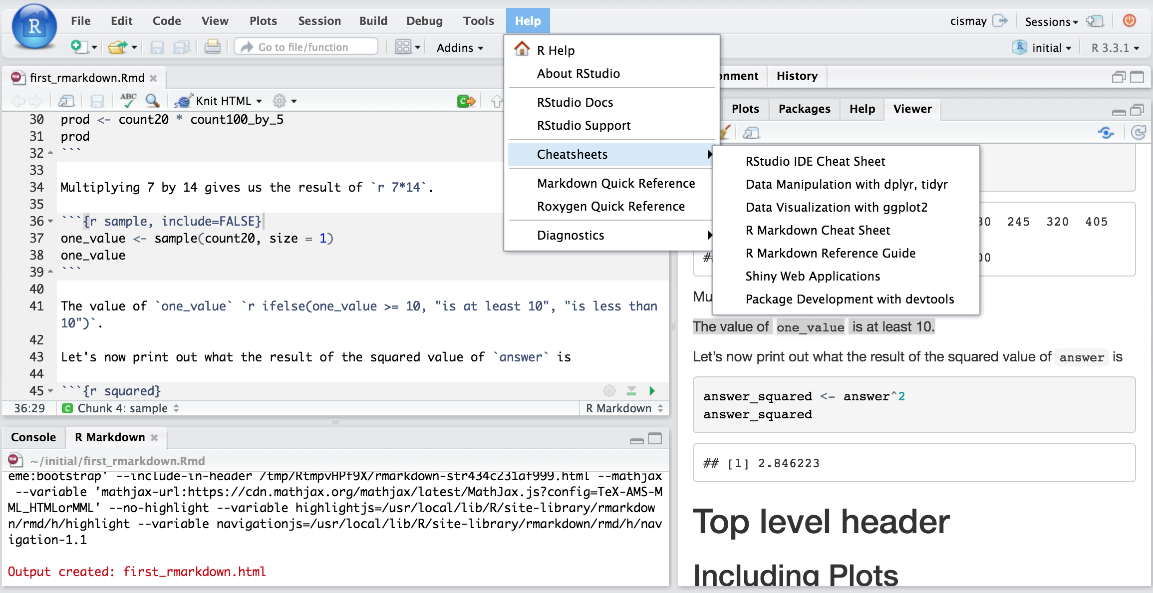
Figure 4.12: RStudio Cheatsheets Screenshot

4.6 Spell-check

Near the top of your R Markdown editor window sits one of the more useful tools for writing documents: the spell-check button. It is the green check-mark with “ABC” above it:

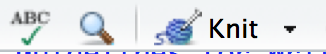
Before you submit a document or share it with someone else, please run a spell-check of your document. You’ll need to add some R commands to the dictionary or ignore them since those may not be words, but it is easy to misspell words as we type and this feature can really help.

---

2. Unless you want to have a fourth, fifth, or sixth level header, but these are not common.↩